


- Accueil
- 80 (2023/1) - Estimer les changements climatiques ...
- Inclusion of a new radiative transfer scheme in the MAR model and validation on Belgium


Visualisation(s): 111 (7 ULiège)
Téléchargement(s): 4 (0 ULiège)

Inclusion of a new radiative transfer scheme in the MAR model and validation on Belgium

Document(s) associé(s)
Version PDF originaleRésumé
Le modèle MAR (Modèle Atmosphérique Régional) est un modèle de climat régional qui a notamment été utilisé pour étudier l’évolution du climat dans les régions polaires, grâce à sa modélisation précise des précipitations et son couplage intégral avec un modèle de neige. Les recherches impliquant MAR ont toutefois occasionnellement souffert des limites de son modèle de transfert radiatif actuel, à savoir le modèle de Morcrette, notamment utilisé par les réanalyses ERA-40 de 2005. Utilisé dans MAR, ce modèle a tendance à tantôt sous-estimer, tantôt surestimer les flux radiatifs descendants en surface. Pour pallier à terme à ces problèmes, cette publication détaille l’inclusion dans le modèle MAR d’ecRad, le dernier schéma de transfert radiatif en date de l’ECMWF. L’année 2011 est simulée sur la Belgique par une version modifiée de MAR v3.13 incluant ecRad afin de valider celle-ci. Les sorties du MAR modifié sont comparées à la fois à des observations collectées par 17 stations météo belges et aux sorties du MAR v3.13 standard utilisant le modèle de Morcrette. Enfin, différentes configurations d’ecRad sont également testées pour évaluer leurs effets respectifs sur le MAR et leurs perspectives.
Abstract
The MAR model (Modèle Atmosphérique Régional) is a regional climate model that has notably been used to study the evolution of the climate in polar areas thanks to its accurate modeling of precipitation and its full coupling to a snow model. Research involving MAR has however occasionally suffered from the limitations of its current radiative transfer scheme, the Morcrette scheme, notably used for the ERA-40 reanalysis (2005). Within MAR, this scheme tends to either underestimate or overestimate the surface downward radiative fluxes. To eventually overcome these limitations, this paper discusses the inclusion in the MAR model of ecRad, the current lattest radiative transfer scheme provided by the ECMWF. The year 2011 is simulated over Belgium by a modified version of MAR v3.13 embedding ecRad in order to validate it. The outputs of the modified MAR are compared both to observations collected by 17 Belgian weather stations in 2011 and to outputs of the standard MAR v3.13., i.e. running with the Morcrette scheme. Finally, various configurations of ecRad are also tested to assess their respective effects on MAR and the prospects they offer.
Table des matières
Introduction
1The MAR model (for Modèle Atmosphérique Régional) is a grid-based regional climate model that has been developped since the middle of the 1990’s (Gallée and Schayes, 1994) in order to research the climate of specific regions at high resolution. A single MAR surface grid point covers a square area whose side is typically a few kilometers long (e.g., 5 kilometers or less for the highest resolutions). While MAR has been used to study various regions over periods of time covering a few years up to several decades (Fettweis et al., 2013a), its development has been driven to put a focus on polar areas: for example, it has been coupled with a snow model in the early 2000’s to study the surface mass balance of the Greenland ice sheet (Gallée and Duynkerke, 1997 ; Lefevre et al., 2003, 2005). Since then, MAR has been run to estimate the future impact of the Greenland ice sheet on sea level rise (Fettweis et al., 2013b) as well as to study the evolution of its surface temperatures (Hanna et al., 2020 ; Delhasse et al., 2020). MAR is also frequently run to study the Antartic ice sheet (Amory et al., 2021 ; C. Kittel, 2021) as well as the evolution of precipitation in various regions, such as Israël (De Ridder and Gallée, 1998), Western Africa (Gallée et al., 2004), equatorial Africa (Doutreloup, 2019), France (Ménégoz et al., 2020), and Belgium (Wyard et al., 2020).
2One of the key components of the MAR model is its radiative transfer scheme (or radiation scheme). The purpose of such a component is to simulate how the energy coming from solar radiation spreads itself across the atmosphere, as well as to simulate the subsequent longwave (or infrared) radiation that results from the Earth’s surface being heated, taking account of surface albedo, greenhouse gases and aerosols in the process. Having an accurate radiative transfer scheme is crucial for a computer climate model, as how the energy flows within the atmosphere and over the surface is ultimately what drives the Earth’s climate. MAR currently uses the radiative transfer scheme by Morcrette (1991, 2002), which has been notably used for the ERA-40 reanalyses (Uppala et al., 2005). It consists in two separate schemes, respectively for shortwave (or solar) radiation and longwave (or infrared) radiation.
3Developed from the 1990’s to the early 2000’s, the Morcrette scheme is now quite old and has well known issues within MAR. In addition to a source code that lacks modularity, as it pre-dates Fortran 2003 (Adams et al., 2009), this scheme also has a tendency to underestimate or overestimate surface downward fluxes in MAR, as evidenced by Fettweis et al. (2017), Delhasse et al. (2020) and Kittel et al. (2022; see also C. Kittel’s PhD thesis, 2021). The MAR model partially compensates for this by making various input and output adjustements, such as operating a small trade-off between shortwave and longwave output fluxes, depending on the region over which it is run.
4This paper discusses the inclusion in the MAR model of a new radiative transfer scheme: the ecRad radiation scheme (Hogan and Bozzo, 2018), the lattest radiative transfer scheme developped by the European Center for Medium-Range Weather Forecasts (ECMWF). Operational since 2017, the ecRad scheme is notably used as the radiation component of the operational weather forecast model of the ECMWF: the IFS (Integrated Forecasting System). The key feature of ecRad is its modularity: its architecture allows users to change independently, among others, the description of optical properties with respects to clouds, greenhouse gases and aerosols, or the radiation equation solver (Hogan and Bozzo, 2018). Compared to the Morcrette scheme still used by MAR v3.13, the ecRad scheme also has the advantage of relying on a collection of NetCDF files to manage gas and aerosol mixing ratios and gas-optics properties. This latter feature comes with two benefits: on the one hand, users can fine tune mixing ratios using the data of their choice, and on the other hand, thanks to recent development, the ecRad scheme is compatible with fine tuned gas-optics models built by ecCKD (Hogan and Matricardi, 2022). Including the ecRad scheme in the MAR model may thus provide multiple benefits, both from a scientific perspective and from a practical point of view.
5The paper is organized as follows. Section I first provides an overview of the ecRad radiation scheme by detailing its initial motivations and main options. Section II subsequently discusses how the MAR model v3.13 has been modified to include ecRad. Section III then validates the modified MAR v3.13 by simulating 2011 over Belgium with it, using observations collected that year by 17 weather stations scattered across Belgium. In the process, outputs of the modified MAR are also compared to those of the standard MAR v3.13 (i.e., running with Morcrette), as well as to those of different configurations of ecRad. Finally, a conclusion summarizes the contributions and perspectives of this research.
I. The ecrad radiation scheme
6This section provides an overview of the ecRad radiation scheme. Section I.A first provides a summary of the development history behind ecRad in order to highlight the motivations behind it and its advantages. Section I.B then reviews the main options offered by the ecRad radiation scheme that are relevant to MAR users, with some of them being subsequently tested in Section III.
A. Development history and motivations
7The ecRad radiation scheme is the product of several decades of development to improve the radiative transfer scheme used within ECMWF’s model, a.k.a. the IFS (Integrated Forecasting System). Starting from the 1990’s, the IFS used the Morcrette radiation scheme (1991), which itself has gone through several updates up to the early 2000’s in order to incorporate various advances in modeling (Morcrette et al., 2008). One major update of the Morcrette scheme was the inclusion of the Rapid Radiative Transfer Model for GCMs (Mlawer et al., 1997), a.k.a. RRTM-G, a correlated-k model for gas absorption. At the time, RRTM-G was used only to simulate longwave radiation and significantly improved the estimation of surface downward longwave radiation compared to contemporary models (Morcrette, 2002). In 2000, the Morcrette scheme used its own gas-optics scheme for shortwave radiation and RRTM-G for longwave radiation, respectively with 4 and 16 spectral bands, and starting from 2002, it used 6 spectral bands for shortwave radiation (Hogan and Bozzo, 2018). This latter version actually corresponds to the radiation scheme used for the ERA-40 reanalyses (Uppala et al., 2005), and therefore, to the radiation scheme used by the MAR model up to its version 3.13.
8In 2007, the Morcrette scheme in the IFS was replaced by McRad (Morcrette et al., 2008), an improved radiative transfer scheme notably featuring a better representation of surface albedo and RRTM-G for both shortwave and longwave radiation (respectively with 14 and 16 spectral bands). It also embeds the Monte-Carlo Independent Column Approximation scheme (McICA), a radiation equation solver that uses a stochastic generator to simulate clouds (Pincus et al., 2003).
9While McRad was a significant improvement with respects to the Morcrette scheme (Morcrette et al., 2008), its source code provided little modularity, making it difficult to include alternative or improved schemes. For instance, climate scientists may want to solve radiation equations with an alternative to the McICA scheme (Pincus et al., 2003). The recent SPARTACUS (SPeedy Algorithm for Radiative Transfer through Cloud Sides) scheme is such an alternative, having notably the ability to simulate 3-D cloud longwave radiative effects (Schäfer et al., 2016; Hogan et al., 2016).
10Another major component of a radiative transfer scheme that may be subject to experimentations is the treatment of the optical properties of gases. Since the early 2000’s, both the IFS and MAR have used the RRTM-G scheme (Mlawer et al., 1997) as their gas-optics model for longwave radiation, and the former started using RRTM-G for shortwave radiation as well in 2007, with the introduction of McRad (Morcrette et al., 2008). A promising alternative to this historic solution is ecCKD (Hogan and Matricardi, 2022), a free tool from the ECMWF that builds fine tuned and computationally efficient gas-optics models via the correlated k-distribution (or CKD) method (Goody et al., 1989).
11The ecRad radiation scheme (Hogan and Bozzo, 2018) was designed to provide the modularity lacking from the McRad scheme, allowing users to easily try out various solutions to manage gas-optics or to solve radiation equations (among others), and paving the way for adding more schemes in the future. Organized in several components through which physical variables transit via dedicated structures, the ecRad scheme lets users pick the scheme of their choice within each component without breaking the flow of the whole radiative transfer scheme. It is worth noting that another goal of ecRad was to improve performance with respects to McRad: the implementation of McICA in McRad constrained the encompassing IFS, used for operational weather forecasting, into running the radiative transfer scheme every 3 hours inside the model, degrading forecasting accuracy in the process. The ecRad radiation scheme provides an improved implementation of McICA that is 41% more efficient than in McRad, allowing for more frequent calls of the scheme (Hogan and Bozzo, 2018).
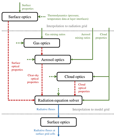
Figure 1. A high-level view of the architecture of the ecRad radiation scheme (based on Figure 1 from Hogan and Bozzo, 2018). Green and blue arrows represent respectively inputs and outputs, while red arrows correspond to optical properties computed by ecRad internal components. Dashed green arrows depict temperature and pressure data at each layer interface that is passed to each component of ecRad.
12Figure 1 illustrates, as a flow-chart, a high-level view of the architecture of the ecRad radiation scheme, where the rectangular boxes depict components of the scheme while the arrows represent the data structures that are flowing from one component to another. This schematic view of the ecRad radiation scheme emphasizes the fact that individual components of the scheme could be any existing method. For example, in the lattest version of ecRad, the radiation equation solver could be either McICA (Pincus et al., 2003), Tripleclouds (Shonk and Hogan, 2008) or SPARTACUS (Schäfer et al., 2016; Hogan et al., 2016), with or without simulating the 3-D radiative effects of clouds. Any choice among these schemes would not require any change with respects to the other components. The lattest build of the ecRad scheme also already allows to swap the classical RRTM-G scheme (Mlwaver et al., 1997) with a gas-optics model built by ecCKD (Hogan and Matricardi, 2022), both in the shortwave and the longwave.
B. Main configuration options
13Thanks to its modularity, the ecRad radiation scheme provides numerous options for users to experiment with. This paper will not cover exhaustively all these options, as Hogan and Bozzo (2018) already provides an inventory of the most important schemes, and will rather focus on those that MAR users are the most likely to want to tune after replacing the Morcrette scheme with ecRad.
14Among the five main components of ecRad (Figure 1), two could be particularily interesting for tuning the MAR model after embedding ecRad. First, the gas-optics component should be tunable by MAR users to create new outputs providing fine spectral data that could be used as forcings by an ocean or vegetation model. Indeed, the RRTM-G scheme as implemented in ecRad uses fixed spectral bands, 14 in the shortwave and 16 in the longwave, and furthermore, the shortwave bands may be too wide to create sound forcings for an ocean or vegetation model that requires spectral data in the photosynthetically active range of shortwave radiation (400 to 700 nm). In particular, one spectral interval of RRTM-G for shortwave radiation in ecRad ranges from 442 to 625 nm, therefore covering almost two thirds of the photosynthetically active range. Since the lattest build of ecRad is already compatible with gas-optics models built by ecCKD (Hogan and Matricardi, 2022), an updated MAR model including ecRad would already be technically able to output fine spectral data to envision future couplings with other computer models. However, ecCKD is still a novelty, and some of the sample models provided by the ECMWF have yet to be validated within a climate simulation.
15The second component of the ecRad radiation scheme MAR users would want to tune is the radiation equation solver. The lattest build of ecRad already provides four schemes for this component: McICA (Pincus et al., 2003), Tripleclouds (Shonk and Hogan, 2008) and SPARTACUS (Schäfer et al., 2016; Hogan et al., 2016) with or without 3-D cloud longwave radiation. The McICA scheme is the solver by default, and is the preferred solution for operational weather forecasting. Though its implementation in ecRad is more efficient and features less noise in atmospheric heating rates than previous instances (Hogan and Bozzo, 2018), McICA may not be the most suitable solver to be used within MAR, as MAR is used for research on past and future climate. However, all three other options are sound for research and should be usable by MAR users. Section III will discuss the practical effects of choosing between either of the three aforementioned options.
16It should be noted that the ecRad radiation scheme also includes numerous older schemes for some of its components, but some are unlikely to be favoured by present and future MAR users. One such option is the possibility to choose the aerosol climatology of Tegen et al. (1997), consisting in 6 hydrophobic aerosol species, for the aerosol optics component. Since the ecRad radiation scheme also accepts the Copernicus Atmospheric Monitoring Service (CAMS) specification consisting in 11 hydrophilic or hydrophobic aerosol species (Flemming et al., 2017; Bozzo et al., 2017), which is much more recent, there is little reason for MAR users to keep using the Tegen climatology (still used by the Morcrette scheme). This is why experiments in Section III will always use this latter option, with the exception of the experiments relying on the Morcrette scheme since it can only run with the Tegen climatology. Finally, experiments in Section III involving ecRad will also all enable longwave scattering by clouds, as this option of the ecRad scheme only adds an increase of 4% in the computational cost thanks to an efficient implementation (Hogan and Bozzo, 2018).
II. Including ecRad in the MAR model
17Written in Fortran 2003 (Adams et al., 2009), the ecRad radiation scheme consists in about 16,000 lines of code without counting the source code of the RRTM-G scheme (Hogan and Bozzo, 2018). It is freely available online on the ECMWF Confluence Wiki (Hogan, 2023b) as a stand-alone software that can be run outside any climate model, and is also freely available on GitHub (Hogan, 2023a). Regardless of where ecRad is downloaded, it also comes with excerpts from the IFS source code to show how the ecRad radiation scheme is initialized then run throughout an IFS simulation.
18Using the ecRad radiation scheme within the MAR model required no modification to the source code of the former. However, interfacing the latter with the former required some work. Section II.A first reviews the forcings expected by the ecRad scheme to highlight the differences with those that already exist in the MAR model, then details how the missing forcings have been implemented. Section II.B subsequently provides a few comments on the methodology followed to progressively include the ecRad radiation scheme in the MAR model as well as on how specific technical aspects of the interfacing have been managed during the process.
A. Updating MAR forcings for ecRad
19Due to the development history of ecRad and the IFS (cf. Section I.A), the example subroutines from the IFS share many input/output variables in common with the subroutines used by MAR (up to version 3.13) to call the Morcrette scheme. Among others, the input variables of the IFS subroutine that calls ecRad include the same description of pressure and temperature as for the Morcrette scheme, and this also holds true for water species mixing ratios and various surface variables (e.g., in terms of albedo, emissivity in the longwave or land/sea mask). However, the ecRad radiation scheme also requires more elaborate inputs when it comes to greenhouse gases and aerosols. Indeed, for each greenhouse gas or aerosol, ecRad needs a volume or mass mixing ratio for each pressure level of each air column of the grid used by the encompassing model. On the other hand, the Morcrette scheme requires such an input only for ozone: other greenhouse gases are forced in a simpler manner (i.e., single mass mixing ratio for the whole atmosphere) or via internal, hard-coded data.
20Therefore, to fully take advantage of the ecRad radiation scheme, the MAR model required updated greenhouse gases and aerosols forcings. Hopefully, the aforementioned ECMWF Confluence Wiki (Hogan, 2023b) also provides the climatological data used by the IFS (cycle 46r1) as additional NetCDF files. The greenhouse gas forcings come as volume mixing ratios averaged with respects to longitude and to each month. These forcings thus consist in twelve 2-D grids (one per month) providing a longitudinal slice of the Earth’s atmosphere with a mixing ratio in each grid point, the data originating from reanalyses covering the 2000’s. Of course, depending on which year the MAR model should simulate, these volume mixing ratios must be scaled to past or future years. One way to do this consists of relying on additional NetCDF files, also provided by the ECMWF, featuring time series of the average volume mixing ratio of each greenhouse gas and for each year (from 0 to 2500) according to the scenarios of the IPCC (Hogan, 2023b). The values from the selected time series corresponding to the years covered by the unmodified forcings are averaged, and the value for the target year (i.e., the year that is simulated by MAR) is divided by that average to compute a scaling factor applied to all grid points of the forcings after selecting the month the MAR will simulate.
21Scaling the forcings to a specific year based on a RCP/SSP scenario is only the first step, as they should also be fitted to the MAR grid. Interestingly, the forcings have a low resolution according to latitude with respects to a MAR grid, but feature a high resolution in terms of pressure levels: the file used in the context of this research (used by the IFS for its cycle 46r1) indeed features 91 pressure levels, which is much higher than the typical number of pressure levels used in the MAR model (24 levels), but has only 64 air columns between both poles. This means, in practice, that a MAR grid will be covered by only a few of the air columns modeled in the forcings. Furthermore, just like the forcings themselves, the volume mixing ratios adjusted to a MAR grid will also be a 2-D longitudinal slice that can be used for all slices of the grid. A simple solution to fit the forcings to the MAR grid therefore consists of picking the air columns closest in latitude to MAR grid points from a same longitudinal slice, then pick the (typically 24) values along each air column that are the closest to the MAR pressure levels. The selected values are finally averaged along the horizontal axis as there is a low number of unique values. The longitudinal slice picked in the MAR grid is currently the slice that includes the air column with the highest surface pressure at the start of the MAR run (one run simulates up to half a month, a new run being automatically scheduled to continue the simulation). The latitudes of the selected slice are used to pick the closest air columns from the forcings while the column with the highest surface pressure is processed to compute the pressure levels (MAR using sigma coordinates) used to select the closest pressure levels from the forcings.
22To illustrate the aforementioned technique, Figure 2 shows an example of a 2-D grid providing volume mixing ratios for carbon dioxide for a longitudinal slice of the Earth’s atmosphere after scaling the values to April 2011. Using the same color scale as Figure 2, Figure 3 illustrates the values that are retained for a MAR grid that covers Belgium and neighboring countries, with latitude ranging from about 49N to about 52.5N, which means that only two columns from the forcings (partly) cover the MAR grid. It is important to point out that the data retained for the MAR grid only covers two thirds of the range of values from the initial air columns because the first 30 pressure levels in the forcings (starting from top of the atmosphere) correspond to very low pressures, while the highest pressure level in a MAR grid is typically around (or a bit below) 100 hPa, i.e., at the top of the troposphere.
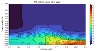
Figure 2. Volume mixing ratios of carbon dioxide for a longitudinal slice of the Earth’s atmosphere, averaged over longitude and scaled to April 2011 (using CMIP6 SSP 370 time series).
23Preparing the new aerosol forcings with respects to the MAR grid is done essentially in the same manner as the greenhouse gas forcings. The main change is that the data (CAMS data also provided by the ECMWF) no longer consists in longitudinal slices, but in 3-D grids (one per month) covering the Earth’s atmosphere in its entirety. Hopefully, again, the low resolution of the forcings allows for some simplifications, as only a few air columns will be covering the high resolution MAR grid. To ease the preparation of the aerosol forcings, the average longitude of the MAR grid points is computed in order to select a single longitudinal slice within the 3-D CAMS data. The rest of the preparation of the forcings then goes exactly like for greenhouse gases. As a result, the MAR model can feed the ecRad radiation scheme with convenient 2-D longitudinal slices of greenhouse gas and aerosol forcings that are adjusted to a specific month and year and to its grid. It should be noted that this way of preparing forcings is not definitive, as other data sources (e.g., with a higher resolution) or other MAR use cases may require a more elaborate approach. However, the resolution of the MAR grids discussed in this paper is high enough, compared to the resolution of the forcings, to justify the described approach.
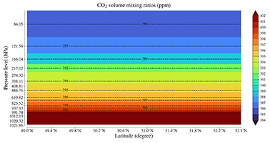
Figure 3. Same volume mixing ratios of carbon dioxide as in Figure 2, but fitted to a MAR grid covering Belgium (cf. Figure 4). The mixing ratios were horizontally averaged. Pressure levels were derived from MAR sigma coordinates and the air column with the highest surface pressure at start.
B. Comments on embedding ecRad in MAR
24While updating the greenhouse gas and aerosol forcings was the most pressing addition to bring to the MAR model in order to include the ecRad radiation scheme, several other modifications of and additions to the MAR source code were required to include ecRad in a smooth manner. First of all, the excerpts from the IFS source code provided along the ecRad radiation scheme (Hogan, 2023a, 2023b) were reused to set up and call it from within the MAR model, with a few minor changes and additions to account for implementation differences between both models (e.g., to access specific parameters and constants). More importantly, the ecRad radiation scheme was not included in the MAR model straight away after updating the forcings (cf. Section II.A) and adapting IFS code excerpts: the entire code for interfacing MAR and ecRad was first tested outside of the former while keeping the latter, using sample data produced with the former as input variables.
25On the one hand, this approach eased the formatting of the MAR variables for ecRad (when necessary) and made it very easy to check at each step that the output variables of the ecRad radiation scheme were consistent with the data it was provided with. On the other hand, it also allowed to tailor aspects of the ecRad embedding that could have led to incoherent MAR outputs if they had been poorly implemented. One of these aspects was how the ecRad radiation scheme was run on the entire MAR grid while using multiple CPUs to speed up execution time. The unmodified MAR model typically calls its radiation scheme on each air column, using OpenMP to distribute the work among multiple CPUs (Fettweis et al., 2017).
26The approach to run ecRad on the MAR grid is slightly different: due to several inputs (like forcings, cf. Section II.A) being formatted as longitudinal slices with respects to the MAR grid, ecRad is called on one longitudinal slice at once, sweeping the grid from the westmost slice to the eastmost one, but blocks of juxtaposed air columns within a slice can be distributed between multiple parallel processes, again with OpenMP. The design of ecRad indeed allows such a parallel distribution, and in fact, this approach is followed by the “offline driver” of ecRad, i.e., the piece of software provided along ecRad itself by the ECMWF to run and test the ecRad radiation scheme outside of any climate model (Hogan, 2023b). Due to the simplicity of the approach, which did not require any modification of ecRad itself, it was re-used to fully process a MAR grid in parallel.
27Finally, a significant amount of time was spent on writing a few additional modules to control the most important options of the ecRad radiation scheme while included in the MAR model and to be able to save some of its variables in separate NetCDF files. Indeed, MAR only needs the clear-sky and total-sky shortwave and longwave radiative fluxes at each pressure level, but ecRad and code from the IFS excerpts can be used to produce additional fluxes, such as the photosynthetically active part of the surface shortwave fluxes or the direct part of the same fluxes. The additional modules offer the possibility to save these additional fluxes in an optional separate NetCDF file. Likewise, they also allow saving the greenhouse gas and aerosol forcings in additional NetCDF files to ensure MAR users can verify these forcings or simply include them in an analysis of MAR results (in fact, Figure 2 and Figure 3 were created this way). All these optional features, as well as the schemes used by ecRad, can be controlled via a configuration file specifically used by the embedded ecRad, and separate from the MAR configuration files. A future version of MAR will provide a default ecRad configuration for each region, letting users fine tune ecRad and control additional output files via a dedicated module.
III. Validation on Belgium
28The ability of the MAR model to accurately simulate the climate of Belgium while using the ecRad radiation scheme is now assessed. Section III.A first reviews the details of the validation process: the data used to validate the results, the configuration of the MAR grid, and the options of the ecRad radiation scheme that were tested. Section III.B subsequently presents and discusses the results. Finally, Section III.C shortly reviews the impact of the inclusion of ecRad on MAR performance.
A. Validation methodology
29Meteorological data recorded throughout 2011 has been used to validate the output variables of the MAR model, both before and after including the ecRad radiation scheme. The data consists of daily means for temperature, shortwave and longwave radiative fluxes as well as daily total of precipitation (combining rainfall and snowfall) recorded by 17 weather stations scattered across Belgium, among which 14 only recorded temperature and precipitation, while 2 recorded all aforementioned variables and the last one recorded all variables except the daily total of precipitation. The locations of the weather stations include, among others, several coastal towns (such as Ostende and Koksijde) and places close to major cities (such as Uccle for Brussels and Bierset airport for Liège), with the southmost station being Buzenol (located south of the province of Luxembourg) and the highest station in altitude being Mont Rigi (located at an altitude of around 660 meters). Finally, it should be noted that the data is exclusively based on raw measurements, i.e., it has not been correlated to other observations nor reanalyzed to mitigate potential measurement biases or errors.
30To perform the validation, multiple simulations have been planned with MAR v3.13, i.e. the lattest version of the MAR model at the time of writing, on a regional grid encompassing Belgium. The grid is of course centered on Belgium, but slightly tilted with respect to the latitude axis in order to ensure Belgium is well enclosed inside the grid, dozens of kilometers separating the Belgian borders from the borders of the grid. Such a configuration maximizes accuracy in simulating precipitation, as the MAR model generates its clouds at the borders of its grid, meaning precipitation will be the most accurately simulated within an inner grid. Finally, this configuration also has the advantage of allowing the use of relatively small grid despite a resolution of 5 kilometers (i.e., a surface grid point covers a 5 by 5 kilometers square area): 120 (longitude-wise) by 90 (latitude-wise) by 24 (pressure levels).
31The forcings for all MAR simulations discussed in this paper have been generated using the NCEP-NCAR reanalysis dataset (Wyszkowski, 2006), but with some topographical correction. Indeed, to ensure the elevation of MAR grid points stays faithful to the altitude of the weather stations, some parts of the grid have been manually adjusted while preparing the forcings to closely match with the real life elevation of the stations, and in particular those located at the highest altitudes (such as Mont Rigi and Saint-Hubert, respectively above 600 and around 500 meters). Finally, the forcings (and therefore, the simulations) cover not only the entire 2011 year but also the last four months of 2010, and this to ensure MAR has been running stably for a while before starting 2011. Figure 4 illustrates the regional grid used for the validation, with the colors and dashed contours describing the elevation.
32A total of six simulations have been carried out. The first two ran with the standard MAR v3.13, i.e. still using the Morcrette radiation scheme, respectively without and with the MAR corrections that make up for the limitations of said scheme. When running over Belgium (and Europe in general), the standard MAR v3.13 applies the following corrections: increasing the surface downward longwave heat fluxes by +1 W/m², substracting 3% of these (increased) fluxes multiplied by 3 to the surface downward shortwave heat fluxes, and finally raising the surface downward longwave heat fluxes by +3%. All heat fluxes are initially deduced from the output variables of the radiation scheme.
33The four remaining simulations ran with the ecRad radiation scheme, without any correction and using specific options each time. As discussed in Section I.A, one advantage of ecRad is its ability to use any scheme within a component of its architecture as long as the data structures stay the same. This capability was therefore also assessed during this research. As discussed in Section I.B, MAR users may wish to tune two specific components of ecRad: the gas-optics model and the radiation equation solver. In particular, being able to use a gas-optics model more refined than RRTM-G (Mlawer et al., 1997) may prove crucial for future MAR uses that would require fine spectral data.
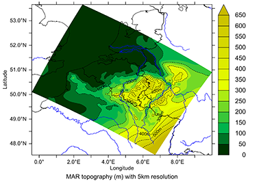
Figure 4. Regional grid used for all six MAR simulations discussed in this paper. The color scale and the dashed contours describe the elevation. Grid points have a resolution of 5 by 5 kilometers.
34The first MAR simulation running with ecRad involves RRTM-G for the gas-optics model and Tripleclouds (Shonk and Hogan, 2008) for solving radiation equations. Both are the oldest schemes available for their respective task, if we omit the McICA solver (Pincus et al., 2003) which is tailored for operational weather forecasting. The second MAR/ecRad simulation also relies on Tripleclouds, but uses ecCKD gas-optics models (Hogan and Matricardi, 2022) rather than RRTM-G. As mentioned earlier (Section I.B), ecCKD offers a promising alternative to RRTM-G but has yet to be validated within a climate model. As such, this second MAR/ecRad simulation is also a validation of ecCKD gas-optics models. For testing’s sake, the most refined models currently provided on the ecRad GitHub (Hogan, 2023a) were used in this simulation, featuring 96 and 64 spectral intervals, or g-points (Morcrette et al., 2008), respectively for shortwave and longwave radiation. The last two simulations with MAR/ecRad are alternatives to the first one, as they both also use RRTM-G but assess the effects of using the more recent SPARTACUS solver (Schäfer et al., 2016; Hogan et al., 2016), with or without 3-D longwave radiative effects of clouds. Table 1 summarizes all configurations.
|
N° |
Radiation scheme |
Gas model |
Solver |
Additional notes |
|
1 |
Morcrette |
RRTM-G (bands: 6 SW, 16 LW) |
Morcrette |
Without MAR corrections |
|
2 |
Morcrette |
RRTM-G (bands: 6 SW, 16 LW) |
Morcrette |
With MAR corrections |
|
3 |
ecRad |
RRTM-G (bands: 14 SW, 16 LW) |
Tripleclouds |
|
|
4 |
ecRad |
ecCKD (g-points: 96 SW, 64 LW) |
Tripleclouds |
|
|
5 |
ecRad |
RRTM-G (bands: 14 SW, 16 LW) |
SPARTACUS |
|
|
6 |
ecRad |
RRTM-G (bands: 14 SW, 16 LW) |
SPARTACUS |
Enabling 3-D cloud effects |
Table 1. Summary of the simulations used to validate MAR v3.13 with or without ecRad. All ran over Belgium (Figure 4) from September 2010 to December 2011 (SW = shortwave, LW = longwave).
B. Validation results
35The output variables of each simulation have been compared to the meteorological data recorded by the 17 weather stations by using, for each station, the time series computed by the MAR model for the (surface) grid point that encompasses the real life location of the station. Then, the bias, root mean square error (or RMSE) and correlation of the MAR time series have been computed for each station. Finally, these statistics have been averaged with respects to the number of stations for which data was available, i.e., temperature statistics have been averaged over the 17 stations, precipitation statistics have been averaged over 16 stations, and finally, longwave and shortwave statistics have been averaged over the 3 stations that recorded radiative fluxes (Buzenol, Dourbes and Retie). The final statistics are provided in Table 2, where the six simulations are listed in the same order as in Table 1.
|
MAR/Morcrette |
MAR/ecRad |
||||||
|
Variable |
Statistic |
N°1 |
N°2 |
N°3 |
N°4 |
N°5 |
N°6 |
|
Temperature (°C) |
Bias |
-0.10 |
-0.10 |
00.14 |
00.13 |
00.14 |
00.17 |
|
RMSE |
01.30 |
01.28 |
01.29 |
01.29 |
01.30 |
01.30 |
|
|
Correlation |
98.12% |
98.12% |
98.29% |
98.29% |
98.29% |
98.29% |
|
|
Precipitations (mm) |
Bias |
00.39 |
00.38 |
00.40 |
00.39 |
00.42 |
00.40 |
|
RMSE |
03.40 |
03.38 |
03.37 |
03.37 |
03.38 |
03.39 |
|
|
Correlation |
63.12% |
63.31% |
64.06% |
63.88% |
64.19% |
63.69% |
|
|
Shortwave (W.m-2) |
Bias |
09.89 |
01.37 |
23.75 |
22.78 |
23.44 |
23.47 |
|
RMSE |
45.07 |
41.74 |
48.94 |
48.03 |
48.92 |
48.81 |
|
|
Correlation |
90.33% |
90.33% |
90.00% |
90.00% |
90.00% |
89.67% |
|
|
Longwave (W.m-2) |
Bias |
05.74 |
11.51 |
00.79 |
00.59 |
00.75 |
01.58 |
|
RMSE |
31.95 |
32.78 |
30.64 |
30.68 |
30.62 |
30.35 |
|
|
Correlation |
78.67% |
79.00% |
80.00% |
80.67% |
80.33% |
80.67% |
|
Table 2. Statistics (averaged) for four MAR output variables, computed with respects to observations recorded in 2011 by 17 weather stations scattered across Belgium. The temperature, shortwave and longwave variables are daily means while the precipitation variable gives daily totals.
36The main highlight from Table 2 is that replacing the old radiation scheme of the MAR model with the ecRad radiation scheme has no negative effect on predicting temperature and precipitation. In fact, the correlation numbers are marginally better with all MAR simulations using ecRad, with an average increase of +0.64% for precipitation with respects to the MAR v3.13 simulation with corrections and of +0.835% without. Such a result is especially a good news for the MAR/ecRad simulation that used ecCKD gas-optics models (Hogan and Matricardi, 2022), as it demonstrates that replacing the old RRTM-G gas-optics model with new, much finer gas-optics models does not negatively impact MAR results, at least in the case of Belgium. Indeed, the temperature and precipitation statistics for the second MAR/ecRad configuration are slightly better than both simulations still using the Morcrette scheme and almost identical to the first MAR/ecRad configuration (with RRTM-G).
37The statistics for the daily means of shortwave and longwave radiative fluxes, on the other hand, require some caution in the analysis: for reminders, only three weather stations recorded such data. A first glance at the average biases for longwave radiative fluxes may suggest using the ecRad radiation scheme significantly reduces the biases for longwave radiation. In practice, the low average biases are due to the results of all MAR/ecRad simulations but the last one having a positive bias of around 14.5 W/m² with respects to Buzenol and negative biases from -6.51 to -5.78 W/m² with respects to the other two stations (Dourbes and Retie). Rather than fixing the biases, using ecRad shifts them with respects to the MAR/Morcrette simulations. This shift amounts to around -5 W/m² with respects to the MAR/Morcrette simulation without corrections, and to around -11 W/m² with respects to the simulation with corrections. In particular, these latter simulations exhibit a bias of respectively +19.63 and +25.59 W/m² with respects to the longwave data from the Buzenol station.
38The MAR/ecRad simulation involving the SPARTACUS solver with 3-D cloud longwave radiative effects enabled exhibits another shift: all biases are shifted by around +1 W/m² with respects to the other MAR/ecRad simulations. The biases become -5.61 and -5.02 W/m² for Dourbes and Retie, respectively, while the bias for Buzenol rises to +15.36 W/m². Such a configuration has thus a subtle, yet noticeable effect on the radiative fluxes in this context. SPARTACUS with 3-D cloud longwave radiative effects may therefore constitute an option to explore depending on the simulated region. Without said 3-D effects, however, the SPARTACUS solver appears to be equivalent to Tripleclouds.
39To deepen the analysis of longwave radiative fluxes, the time series for the observations (daily means) can be compared to those of the longwave radiative fluxes (daily means too) produced by each of the six simulations. In particular, the case of the Buzenol station should be carefully reviewed, as its longwave statistics include, for all simulations, a large positive bias but also a lower correlation (around 64%) than with the two other stations that recorded longwave fluxes. Figure 5 provides the time series of the longwave fluxes in 2011 from both the observations at the Buzenol station and the six MAR simulations (encompassing grid point). For comparison’s sake, Figure 6 provides the same type of figure for the Retie station, for which the correlation was close to 90% in all cases (to compare to the average correlation of around 80% exhibited in Table 2). Finally, for better visualization, Figure 7 and Figure 8 plot the differences (in W/m²) between the MAR time series and the observations of respectively Buzenol and Retie, using the same data and colors as in Figure 5 and 6.
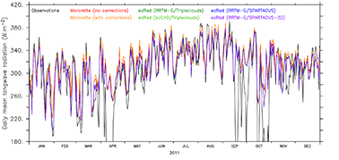
Figure 5. Times series of the daily mean for longwave radiative fluxes at the Buzenol weather station (black) compared to those from the six MAR simulations (encompassing grid point) for 2011.
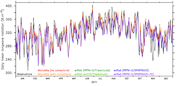
Figure 6. Times series of the daily mean for longwave radiative fluxes at the Retie weather station (black) compared to those from the six MAR simulations (encompassing grid point) for 2011.
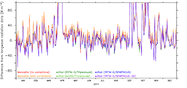
Figure 7. Differences between the time series of Buzenol and the time series from the six MAR simulations (encompassing grid point) for longwave radiation. The data is the same as in Figure 5.
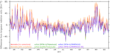
Figure 8. Differences between the time series of Retie and the time series from the six MAR simulations (encompassing grid point) for longwave radiation. The data is the same as in Figure 6.
40The time series depicted in Figure 5 to 8 suggest that there are issues with the measurements from the Buzenol weather station: on several occasions, the daily mean plunges for several days down to near-zero values (which are not shown in Figure 5 to better visualize the other fluctuations). Despite that observations for Retie are also significantly below MAR predictions (regardless of the simulation) on a few occasions (see November 2011 in Figure 6, for instance), the magnitude of the differences with MAR results remain in the order of a few dozens of W/m² while differences in Figure 5 can exceed one or two hundreds W/m². These large differences are further highlighted in Figure 7 and Figure 8, as curves in the former go beyond +100 W/m² on a few occasions while curves in the later never exceed +80 W/m² with most of the time series being comprised between -50 to +50 W/m². The worse statistics for Buzenol station can therefore be assumed to be due to a measurement issue rather than a problem with the radiative transfer schemes used by the MAR model, therefore suggesting that both schemes would correlate significantly higher than 80% with better data, contrary to what Table 2 suggests. However, a difference between both schemes remain: the aforementioned shifts in the biases between the Morcrette radiation scheme and the ecRad radiation scheme can also be observed in both figures. Indeed, the red and orange curves (MAR/Morcrette simulations) are regularly above the curves corresponding to MAR/ecRad simulations, which are themselves very close to each other (if not identical) despite the varying configurations.
41Another shift can also be observed in the biases for shortwave radiative fluxes in Table 2. Indeed, there is a significant increase in the biases for shortwave radiative fluxes (around +20 W/m²) between the MAR/Morcrette and the MAR/ecRad simulations, though the correlation factors remain close or equal to 90% across all simulations. Again, to visualize this shift, the time series for the daily means of shortwave radiative fluxes found in the meteorological data and in the MAR results can be plotted. Figure 9 and Figure 10 illustrate these time series, respectively for the Buzenol and Dourbes weather stations, with the same format as Figure 5 and Figure 6.
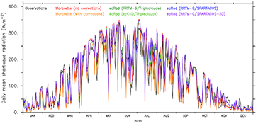
Figure 9. Times series of the daily mean for shortwave radiative fluxes at the Buzenol weather station (black) compared to those from the six MAR simulations (encompassing grid point) for 2011.

Figure 10. Times series of the daily mean for shortwave radiative fluxes at the Dourbes weather station (black) compared to those from the six MAR simulations (encompassing grid point) for 2011.
42This time, the Buzenol data does not appear to feature major measurement errors, and both figures suggest a good correlation between observations and MAR results. A closer look at the figures nevertheless suggest that the ecRad radiation scheme increases the shortwave radiative fluxes: the curves corresponding to MAR/ecRad simulations tend to be above the others (including observations), especially during summer months. To better visualize this shift, Figure 11 and Figure 12 illustrates the differences between the MAR time series and the observations, in the same manner as Figure 7 and 8 but with respects to Figure 9 and 10. In these two last figures, the red and orange curves (MAR/Morcrette simulations) bear most of the local minima, contrary to what was observed in Figure 7 and Figure 8. On the other hand, the local maxima are shared among the MAR/ecRad curves, the largest differences with respects to observations being observed during summer months, as shown in Figure 11 and Figure 12. It is also during these months that differences between the MAR/ecRad simulations become more visible.
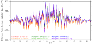
Figure 11. Differences between the time series of Buzenol and the time series from the six MAR simulations (encompassing grid point) for shortwave radiation. The data is the same as in Figure 9.
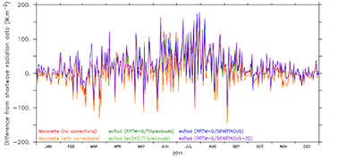
Figure 12. Differences between the time series of Dourbes and the time series from the six MAR simulations (encompassing grid point) for shortwave radiation. The data is the same as in Figure 10.
43There are multiple possible causes to explain why the MAR/ecRad simulations produced significant biases for radiative fluxes, in particular in the shortwave. First of all, the solar constant used to compute insolation is set to 1366 W/m² in the code excerpts from the IFS that have been re-used to interface MAR with ecRad. The standard MAR v3.13 uses a slightly lower constant (1360.8 W/m²) to account for the loss of energy in the upper layers of the atmosphere, since the MAR grid does not usually extend beyond the lower part of the stratosphere. Adjusting this constant for the needs of MAR should therefore reduce shortwave fluxes. Second, the MAR forcings used in this research have been computed with low resolution data (NCEP-NCAR reanalysis; Wyszkowski, 2006): higher resolution data would result in better forcings and better validation results, including for radiative fluxes. Third, and more importantly, underestimated cloud fraction values may play a significant role in inducing large biases. Previous work involving the MAR model already noted that biases obtained with the Morcrette scheme may be due to a lack of cloudiness (Fettweis et al., 2017). In the context of this research, updating how MAR computes cloud fraction values prior to feeding them to its radiation scheme has not been considered, with MAR v3.13 still relying on an old parameterization from the ECMWF to do so. Future work will focus on improving the radiative balance of MAR/ecRad by re-evaluating its way of computing cloud fraction values for ecRad and by better taking account of the effects of the upper atmosphere on radiative fluxes. It will also assess whether or not the heat flux error compensations implemented by MAR v3.13 to mitigate the biases obtained with the Morcrette scheme are still needed to achieve a balanced radiative budget with ecRad.
C. Impact of ecRad on MAR performance
44For completeness’ sake, the impact on execution time of running the MAR model with the ecRad radiation scheme rather than the Mocrette radiation scheme should also be assessed. To do so, the MAR model has been run on a single day over Belgium (grid from Figure 4), first with the standard MAR v3.13 (Morcrette scheme) then with each ecRad configuration from Table 1, and with an increasing number of CPUs: 4, 6 then 8 CPUs. It is assumed the MAR corrections applied after calling the old radiation scheme have a negligible computational cost. Each experiment was timed with the time command of Linux, which notably provides the real time spent by an application outside system calls. For each number of CPUs considered here, Table 3 provides the relative increases in execution time between each ecRad configuration and the standard MAR v3.13, complete with an average. Table 3 also reminds the options used by each ecRad configuration for readability’s sake.
|
ecRad configuration |
First |
Second |
Third |
Fourth |
|
Gas-optics model |
RRTM-G |
ecCKD |
RRTM-G |
RRTM-G |
|
Radiation solver |
Tripleclouds |
Tripleclouds |
SPARTACUS |
SPARTACUS (3D) |
|
Relative increase with 4 CPUs |
+6.16% |
+4.17% |
+8.90% |
+31.40% |
|
Relative increase with 6 CPUs |
+4.47% |
+2.53% |
+8.04% |
+36.99% |
|
Relative increase with 8 CPUs |
+4.86% |
+2.63% |
+6.00% |
+25.59% |
|
Average relative increase |
+5.16% |
+3.11% |
+7.65% |
+31.37% |
Table 3. Comparison of execution times of the MAR model embedding ecRad w.r.t. the unmodified MAR v3.13, based on a single day of simulation and using an increasing number of CPUs.
45Table 3 shows that the simpler configurations of the ecRad radiation scheme led to a marginal increase of the execution times. In particular, the increase for the ecCKD/Tripleclouds configuration is barely exceeding 3% on average, which is likely due to ecRad running a bit faster with gas-optics models built by ecCKD than with RRTM-G. Only the RRTM-G/SPARTACUS-3D configuration led to a substantial increase of around 31% of the total execution time on average. This increase can be explained in at least two ways: on the one hand, the SPARTACUS solver with 3-D cloud longwave radiative effects enabled is the most ambitious scheme currently provided by ecRad for solving radiation equations, and on the other hand, the embedded ecRad had to be compiled with double precision for the 3-D effects to be properly simulated. In all other configurations, ecRad could be compiled with simple precision to reduce memory use. The average relative increase of 7.65% for the RRTM-G/SPARTACUS configuration, which is the second largest average relative increase in Table 3, is also likely due to using the SPARTACUS solver rather than the less recent Tripleclouds solver. A deeper characterization of the performance implications of using the ecRad radiation scheme within the MAR model (and the effects of various schemes) is left for future work.
Conclusion
46Accurately simulating the climate with a computer model is a challenging task whose success partly relies on the accuracy of an underlying radiative transfer scheme, i.e., a model predicting how the shortwave and longwave radiation flows throughout the Earth’s atmosphere. Since the 2000’s, the MAR model has relied on a late version of the Morcrette scheme (1991, 2002) that was notably used for the ERA-40 reanalysis (Uppala et al., 2005). Since then, more exhaustive and/or accurate radiative transfer schemes have been introduced. The ecRad radiation scheme (Hogan and Bozzo, 2018) is the lattest radiative transfer scheme provided by the ECMWF, and distinguishes itself from past schemes by emphasizing modularity to allow its users to swap one inner scheme with another. In particular, the lattest version of ecRad (Hogan, 2023a) is able to replace the classical gas-optics scheme RRTM-G (Mlawer et al., 1997) with fine-tuned models built with the ecCKD tool (Hogan and Matricardi, 2022).
47This paper discussed including the ecRad radiation scheme within the MAR model to eventually replace the old scheme. In addition to reviewing the perspectives of such an update and describing how it was implemented for the first time, this work also provided a first validation of a modified MAR v3.13 running with ecRad over Belgium in 2011, using meteorological data for that year recorded by 17 weather stations scattered across the country. Not only the MAR model embedding the ecRad radiation scheme was validated, but it was also run with varying configurations of the latter in order to assess the effects and perspectives of such configurations. Two additional simulations with the standard MAR model version 3.13 (i.e., running with the Morcrette radiation scheme), respectively without and with heat fluxes errors compensations, were also performed for comparison’s sake.
48Comparison of the results of all the simulations discussed in this work demonstrated that including the ecRad radiation scheme within the MAR model has no negative consequences when it comes to predicting temperature and precipitation. In fact, a marginal increase of the correlation statistics with respects to the precipitation records was even observed with the MAR/ecRad configurations, even though the MAR model has yet to be fully adjusted to ecRad.
49A careful analysis of the radiative fluxes both recorded by Belgian weather stations and computed by the MAR simulations showed that replacing the old radiative transfer scheme with ecRad induced a shift in the biases with respects to the observations, with longwave fluxes being less overestimated than before while the opposite was observed with shortwave fluxes. The large biases obtained for the shortwave fluxes with MAR/ecRad simulations are likely due to MAR not being tuned for its new radiation scheme yet: in particular, a lack of cloudiness, which was already pointed as a possible cause for the biases obtained with the Morcrette scheme by Fettweis et al. (2017), may explain the large biases of the MAR/ecRad simulations, especially during the summer months. Other causes include the higher solar constant found in the code excerpts from the IFS reused to interface MAR with ecRad and the low resolution of the forcings used to prepare the simulations.
50A comparison of the time series coming from both observations and MAR results showed that the data provided by one of the weather stations recording longwave radiation likely included measurement errors, therefore suggesting better data would have led to higher correlation statistics for longwave fluxes for all simulations discussed in this paper.
51When it comes to the different options offered by the ecRad radiation scheme, an important contribution of this work is the validation of ecCKD-built gas-optics models while embedded in a climate model. Indeed, the finer spectral resolution of said gas-optics models may be used to produce fine spectral data with the MAR model, which may be later used as forcings for other computer models, such as ocean or vegetation models, or even for couplings. The other explored options, namely radiation equation solvers, did not have a major impact on MAR results, though the SPARTACUS solver with 3-D cloud longwave radiative effects induced another shift (around +1 W/m² on average) in the longwave radiative fluxes with respects to the observations. This configuration however comes with a greater computational cost than other solvers provided by ecRad.
52Future work will focus on achieving radiative balance with MAR embedding ecRad by improving cloudiness and the effects of the upper atmosphere on radiative fluxes. More exhaustive validations, relying on better MAR forcings and covering longer periods of time and/or other regions, will be carried out for this purpose. The computation, validation and use of spectral radiative fluxes will also be explored on the longer term.
Acknowledgements
53A good part of the research work presented in this paper has been made significantly easier by the active support of Robin J. Hogan, senior scientist at the ECMWF and main developer of the ecRad radiation scheme.
References
54Adams, J., Brainerd, W., Hendrickson, R., Maine, R., Martin, J., and Smith, B. (2003). The Fortran 2003 Handbook. https://doi.org/10.1007/978-1-84628-746-6
55Amory, C., Kittel, C., Le Temoulin, L., Agosta, C., Delhasse, A., Favier, V. & Fettweis, X. (2021). Performance of MAR (v3.11) in simulating the drifting-snow climate and surface mass balance of Adélie Land, East Antarctica. Geoscientific Model Development, 14(6), 3487-3510.
56Bozzo, A., Rémy, S., Benedetti, A., Flemming, J., Bechtold, P., Rodwell, M. & Morcrette, J.-J. (2017). Implementation of a CAMS-based aerosol climatology in the IFS. ECMWF Technical Report 801.
57Delhasse, A., Kittel, C., Amory, C., Hofer, S., van As, D., Fausto R. S. & Fettweis, X. (2020). Evaluation of the near-surface climate in ERA5 over the Greenland Ice Sheet. Cryosphere, 14(3), 957-965.
58De Ridder, K. & Gallée H., (1998). Land Surface-induced regional climate change in Southern Israel. Journal of Applied Meteorology, 37, 1470-1485.
59Doutreloup, S. (2019). Évolution actuelle et future des précipitations convectives sur la Belgique et la région du Lac Victoria (Afrique équatoriale de l’Est) à l’aide du modèle climatique régional MAR. Unpublished doctoral thesis. https://hdl.handle.net/2268/239971
60Fettweis, X., Hanna, E., Lang, C., Belleflamme, A., Erpicum, M. & Gallée, H. (2013a). Important role of the mid-tropospheric atmospheric circulation in the recent surface melt increase over the Greenland ice sheet. Cryosphere, 7(1), 241-248.
61Fettweis, X., Franco, B., Tedesco, M., Van Angelen, J., Lenaerts, J., Van Den Broeke, M. & Gallée, H. (2013b). Estimating the Greenland Ice Sheet surface mass balance contribution to future sea level rise using the regional atmospheric climate model MAR. Cryosphere, 7(2), 469-489.
62Fettweis, X., Box, J., Agosta, C., Amory, C., Kittel, C., Lang, C., van As, D., Machguth, H., & Gallée, H. (2017). Reconstructions of the 1900–2015 Greenland ice sheet surface mass balance using the regional climate MAR model. Cryosphere, 11(2), 1015–1033.
63Flemming, J., Benedetti, A., Inness, A., Engelen, R. J., Jones, L., Huijnen, V., Rémy, S., Parrington, M., Suttie, M., Bozzo, A., Peuch, V.-H., Akritidis, D. & Katragkou, E. (2017). The CAMS interim reanalysis of carbon monoxide, ozone and aerosol for 2003–2015. Atmospheric Chemistry and Physics, 17(3), 1945-1983.
64Gallée, H. & Schayes, G. (1994). Development of a Three-Dimensional Meso-γ Primitive Equation Model: Katabatic Winds Simulation in the Area of Terra Nova Bay, Antarctica. Monthly Weather Review, 122(4), 671–685.
65Gallée, H., & Duynkerke, P. (1997). Air-Snow Interactions and the Surface Energy and Mass Balance over the Melting Zone of West Greenland during GIMEX. Journal of Geophysical Research, 102, 13813-13824.
66Gallée, H., Moufouma-Okia, W., Bechtold, P., Brasseur, O., Dupays, I., Marbaix, P., Messager, C., Ramel, R. & Lebel, T. (2004). A high resolution simulation of a West African rainy season using a regional climate model. Journal of Geophysical Research, 109, D05108.
67Goody, R., West, R., Chen, L., & Crisp, D. (1989). The correlated-k method for radiation calculations in nonhomogeneous atmospheres. Journal of Quantitative Spectroscopy & Radiative Transfer, 42(6), 539–550.
68Hanna, E., Cappelen, J., Fettweis, X., Mernild, S. H., Mote, T. L., Mottram, R., Steffen, K., Ballinger, T. J. & Hall, R. J. (2020). Greenland surface air temperature changes from 1981 to 2019 and implications for ice-sheet melt and mass-balance change. International Journal of Climatology, 41(S1), E1336-E1352.
69Hogan, R. J., Schäfer, S. A. K., Klinger, C., Christine Chiu, J. & Mayer, B. (2016). Representing 3-D cloud radiation effects in two-stream schemes: 2. Matrix formulation and broadband evaluation. Journal of Geophysical Research Atmospheres, 121(14), 8583-8599.
70Hogan, R. J. & Bozzo, A. (2018). A flexible and efficient radiation scheme for the ECMWF model. Journal of Advances in Modeling Earth Systems, 10(8), 1990-2008.
71Hogan, R. J. & Matricardi, M. (2022). A tool for generating fast k-distribution gas-optics models for weather and climate applications. Journal of Advances in Modeling Earth Systems, 14(10), e2022MS003033.
72Hogan, R. J. (2023a). ecmwf-ifs/ecrad: ECRAD - ECMWF atmospheric radiation scheme. GitHub. https://github.com/ecmwf-ifs/ecrad
73Hogan, R. J. (2023b). ECMWF Radiation Scheme Home. ECMWF Confluence Wiki. https://confluence.ecmwf.int/display/ECRAD/
74Kittel, C. (2021). Present and future sensitivity of the Antarctic surface mass balance to oceanic and atmospheric forcings: insights with the regional climate model MAR. PhD thesis. University of Liège, Liège. http://hdl.handle.net/2268/258491
75Kittel, C., Amory, C., Hofer, S., Agosta, C., Jourdain, N. C., Gilbert, E., Le Toumelin, L., Vignon, E., Gallée, H. & Fettweis, X. (2022). Clouds drive differences in future surface melt over the
Antarctic ice shelves. Cryosphere, 16(7), 2655-2669.
76Lefebre, F., Gallée, H., van Ypersele, J., & Greuell, W. (2003). Modeling of snow and ice melt at ETH-camp (West Greenland): a study of surface albedo. Journal of Geophysical Research Atmospheres, 108(D8).
77Lefebre, F., Fettweis, X., Gallée, H., van Ypersele, J., Marbaix, P., Greuell, W., & Calanca, P. (2005). Evaluation of a high-resolution regional climate simulation over Greenland. Climate Dynamics, 25(1), 99-116.
78Ménégoz, M., Valla, E., Jourdain, N. C., Blanchet, J., Beaumet, J., Wilhelm, B., Gallée, H., Fettweis, X., Morin, S., & Anquetin, S. (2020). Contrasting seasonal changes in total and intense precipitation in the European Alps from 1903 to 2010, Hydrol. Earth Syst. Sci., 24, 5355–5377.
79Mlawer, E. J., Taubman, S. J., Brown, P. D., Iacono, M. J. & Clough, S. A. (1997). Radiative transfer for inhomogeneous atmospheres: RRTM, a validated correlated-k model for the longwave. Journal of Geophysical Research Atmospheres, 102(D14), 16663–16682.
80Morcrette, J.-J. (1991). Radiation and cloud radiative properties in the ECMWF operational forecast model. Journal of Geophysical Research Atmospheres, 96, 9121-9132.
81Morcrette, J.-J. (2002). The Surface Downward Longwave Radiation in the ECMWF Forecast System. Journal of Climate, 15(14), 1875-1892.
82Morcrette, J.-J., Barker, H. W., Cole, J. N. S., Iacono, M. J., & Pincus, R. (2008). Impact of a New Radiation Package, McRad, in the ECMWF Integrated Forecasting System. Monthly Weather Review, 136(12), 4773-4798.
83Pincus, R., Barker, H. W., & Morcrette, J.-J. (2003). A fast, flexible, approximate technique for computing radiative transfer in inhomogeneous cloud fields. Journal of Geophysical Research Atmospheres, 108(D13), 4376.
84Schäfer, S. A. K., Hogan, R. J., Klinger, C., Christine Chiu, J. & Mayer, B. (2016). Representing 3-D cloud radiation effects in two-stream schemes: 1. Longwave considerations and effective cloud edge length. Journal of Geophysical Research Atmospheres, 121(14), 8567-8582.
85Shonk, J. K. P. & Hogan, R. J. (2008). Tripleclouds: An Efficient Method for Representing Horizontal Cloud Inhomogeneity in 1D Radiation Schemes by Using Three Regions at Each Height. Journal of Climate, 21(11), 2352–2370.
86Tegen, I., Hollrig, P., Chin, M., Fung, I., Jacob, D., & Penner, J. (1997). Contribution of different aerosol species to the global aerosol extinction optical thickness: Estimates from model results. Journal of Geophysical Research Atmospheres, 102(D20), 23895-23915.
87Uppala, S. M., Kållberg, P., Simmons, A., Andrae, U., Bechtold, V. D. C., Fiorino, M., Gibson, J., Haseler, J., Hernandez, A., Kelly, G., Li, X., Onogo, K., Saarinen, S., Sokka, N., Allan, R. P., Andersson, E., Arpe, K., Balmaseda, M. A., Beljaars, A. C. M., Berg, L. V. D., Bidlot, J., Bormann, N., Caires, S., Chevallier, F., Dethof, A., Dragosavac, M., Fisher, M., Fuentes, M., Hagemann, S., Hólm, E., Hoskins, B. J., Isaksen, L., Janssen, P. A., Jenne, R., Mcnally, A. P., Mahfouf, J. F., Morcrette, J.-J., Rayner, N. A., Saunders, R. W., Simon, P., Sterl, A., Trenberth, K. E., Untch, A., Vasiljevic, D., Viterbo, P. & Woolen, J. (2005). The ERA-40 re-analysis. Quarterly Journal of the Royal Meteorological Society: A journal of the atmospheric sciences, applied meteorology and physical oceanography, 131(612), 2961-3012.
88Wyard, C., Scholzen, C., Doutreloup, S., Hallot, E. & Fettweis, X. (2020). Future evolution of the hydroclimatic conditions favouring floods in the south-east of Belgium by 2100 using a regional climate model, International Journal of Climatology, 41(1), 647-662.
89Wyszkowski, A. (2006). NCEP/NCAR Reanalysis Project - General information, availability and application. Annales Universitatis Mariae Curie-Sklodowska sectio B – Geographia Geologia Mineralogia et Petrographia, 61, 478-487.
Pour citer cet article
A propos de : Jean-François GRAILET
Faculté des Sciences
Département d'astrophysique, géophysique et océanographie (AGO)
MAST (Modeling for Aquatic Systems)
ULiège
jean-francois.grailet@uliege.be