


- Accueil
- Volume 19 (2015)
- Numéro 2
- Evaluation of the “observer effect” in botanical surveys of grasslands


Visualisation(s): 1149 (21 ULiège)
Téléchargement(s): 66 (3 ULiège)

Evaluation of the “observer effect” in botanical surveys of grasslands

Notes de la rédaction
Received on July 4, 2014; accepted on January 9, 2015
Résumé
Évaluation de « l’effet observateur » dans les relevés botaniques en prairies
Description du sujet. Une étude de terrain a été menée sur 24 parcelles de prairies avec cinq experts botanistes afin d’évaluer d’éventuels biais dans les relevés, ainsi que leurs conséquences possibles quant à la description des habitats semi-naturels concernés.
Objectifs. Afin de connaitre les principaux facteurs de variabilité entre observateurs et leur amplitude respective lors de relevés botaniques en prairies, une étude a été menée et les résultats ont été analysés statistiquement. Les résultats ont débouché sur la mise en place de solutions pratiques pour améliorer la qualité des relevés et diminuer la variabilité entre observateurs.
Méthode. Cinq observateurs de terrain ont effectué des relevés botaniques complets sur 24 parcelles de prairies en Famenne (Wallonie, Belgique) en juin 2009. Tous les relevés ont été analysés statistiquement pour détecter et quantifier les différentes sources de variabilité entre observateurs. Les principaux paramètres comparés sont le diagnostic de qualification de l’habitat par les experts, le taux de détection des espèces caractéristiques, ainsi que leur taux de recouvrement sur chaque parcelle.
Résultats. En termes d’identification d’habitat, les différences les plus importantes entre les observateurs ont été constatées dans les parcelles qui avaient une composition intermédiaire entre un habitat typique en bon état de conservation et un habitat nettement dégradé. De manière générale, il a été constaté une légère tendance à la sous-évaluation de la qualité de l’habitat. Les analyses ont révélé que la première cause de variabilité provient du fait que les observateurs ne suivaient pas toujours scrupuleusement les seuils des paramètres utilisés pour l’identification de l’habitat. En ce qui concerne la comparaison entre observateurs, les principales sources de variabilité proviennent des estimations des taux de recouvrement de certaines plantes, des taux de détection des espèces caractéristiques ainsi que de l’effort de prospection qui n’est pas toujours optimal.
Conclusions. Les différentes sources de variabilité qui ont été mises en évidence peuvent soit être réglées facilement, soit devront être gardées à l’esprit lors des comparaisons futures entre relevés. Les principales solutions proposées sont les suivantes : un meilleur contrôle par l’observateur de son travail à toutes les étapes ; une organisation de formations ciblées ; des efforts de prospections standardisés.
Abstract
Description of the subject. A field study has been conducted on 24 grasslands with five different botanical experts in order to assess inter-observer bias when making botanical surveys as well as the possible consequences in terms of descripting a semi-natural habitat.
Objectives. Fieldwork has been conducted to understand the most important factors of variability affecting botanical surveys conducted by several observers. These results were used to suggest practical solutions to enhance the quality of such surveys.
Method. Five observers performed a complete botanical survey of 24 grassland plots in the Famenne (Wallonia, Belgium) in June 2009. All surveys were statistically analyzed in order to detect and quantify the sources of variability between observers. The main parameters compared are the habitat diagnosis made on the field by the experts, the rate of detection of the characteristic species as well as their coverage in each plot.
Results. Regarding habitat identification, the biggest differences between observers are seen in plots where the composition is intermediate between a habitat in good and in bad status. Overall, there was a slight tendency to undervalue the quality of the habitat. The analysis revealed that the primary cause of variability between observers is the fact that the experts did not always strictly follow the criteria for habitat identification. As regards the comparison between observers, several sources of variability were identified. The main ones are the variability of the estimated coverage of some plants, the variability of the detection rate of characteristic species, as well as the variability of the prospecting effort that can be sub-optimal in each plot.
Conclusions. Some of the sources of variability that have been pointed out can be resolved easily, other have to be taken in consideration when comparing the results of surveys in the future. The solutions proposed to reduce the variability between observers are to encourage better self-control of the parameters to be taken into account at each step of the work, the organization of targeted training courses and more standardized prospecting efforts.
Table des matières
1. Introduction
1After acceptance by the European Commission of the limits of Natura 2000 sites in Wallonia between 2002 and 2005, the first step of the implementation of the Natura 2000 network was the detailed mapping of all habitats in the sites before the publication of the official Designation Acts, as well as the evaluation of their conservation degrees at each site (Dufrêne et al., 2013). The degree of conservation integrates parameters such as the structure, the functions and the restoration possibilities at the level of each particular Natura 2000 site. As stated in the Habitats Directive (HD), the aim to be achieved is at least to maintain the conservation status registered at the time of the site's designation. The objective at the regional scale is to maintain a favorable conservation status and if this is not the case, to restore it.
2The identification of the habitats and the assessment of their conservation status by different experts implies providing them with specific tools to reduce the risk of diverging interpretations in the assessments (Bottin et al., 2005). To meet these requirements the Department of the Study of the Natural Environment and Agriculture (DEMNA, formerly CRNFB) of the Public Service of Wallonia collaborated with several universities (ULg, UCL, Gx-ABT formerly FUSAGx). Between 2003 and 2005 technical documents were developed, including identification keys to the habitats on the basis of (for grasslands) lists of “characteristic species” and minimum coverage thresholds. These documents were necessary to identify and assess the conservation status of these habitats (Halford et al., 2006; Legast et al., 2006).
3Since 2002 the WalEUNIS typology (Dufrêne et al., 2005) has been used in Wallonia to refer to different habitats. This typology is a Walloon adaptation of the European EUNIS typology (Davies et al., 2002), which is more detailed and comprehensive than the CORINE one. These WalEUNIS codes are used by the experts to identify whether the habitat falls within any of Habitats of Community Interest (HIC) or not (NHIC) as mentioned in Annex I of the Habitats Directive (EUR28) (European Commission, 2013), using the technical documents mentioned above.
4In this case, the target habitat is “Hay meadows”, named “E2.22” in the WalEUNIS typology and “6510” in the EUR28 (European Commission, 2013) typology. Hay meadows are herbaceous vegetation installed on relatively fertile and well-drained soils. They are traditionally mown in early summer for hay production. Their plant composition includes a wide variety of grasses and forbs, especially in the less fertilized variants. These mesophilic meadows are acutely threatened by agricultural intensification, particularly through the use of fertilizers and/or grazing, but also due to cultivation or abandonment. The direct consequence of their degradation is a general loss of biodiversity. In the field, one can observe a gradient of habitats in good status, habitats in an intermediate status as well as degraded grasslands that can no longer be considered as hay meadows. These are classified using the WalEUNIS typology as “intensive grasslands” named “E2.11a” when intensively grazed or as “heavily fertilized grasslands” named “E2.11c” when intensively used for the production of hay (silage) and grazing. Such meadows are not considered as HICs.
5However, even if field surveys made by our botanical experts were made by using the identification keys for WalEUNIS habitats thus theoretically reducing the inter-experts variability, it is well known that this type of survey is accompanied by variability due to the observer and to the period of year at which the surveys are conducted (Moore et al., 1970; Kirby et al., 1986; Leps et al., 1992; Klimes et al., 2001; Vittoz et al., 2007). When comparing species lists provided by different observers this variability was estimated at 13% in 5 x 5 m grassland quadrats (Klimes et al., 2001) and at more than 10% by Vittoz et al. (2007) on 40 m2 quadrats. For Hope-Simpson (1940), and as later recalled by Scott et al. (2002), it is necessary to make preliminary tests to determine the rate of variability intrinsic to each type of inventory method.
6The main objective of this study is to quantify the “observer” effect, also called “pseudo-turnover”, “false turnover”, “sampling error” or “sampling bias” (according to the authors, see Klimes et al., 2001) that can reasonably be expected in the surveys conducted by different experts analyzing the same fields in the same period of time. In this article, we present the results of the “observer” effect (the analysis of the “season” effect will be treated later on).
7There is a real methodological challenge in evaluating the variation of field diagnosis made by different experts on basis of their botanical surveys and when using the identification keys in these situations of a continuous gradient between grasslands with a high conservation value protected by specific constraints (HIC 6510) and highly degraded grasslands (NHIC) where the constraints are very limited. Indeed it is essential to make a correct evaluation in order to avoid imposing unnecessary or disproportionate constraints to site managers (mainly farmers), but also to protect the unique biological heritage still remaining. In addition, when monitoring the sites every six years as required by the Habitats Directive, it is important to ensure consistency of the diagnosis if the situation has not changed. The reporting of a decline in conservation status either at a Natura 2000 site or at the biogeographical level could trigger significant corrective measures.
2. Methods
2.1. Field surveys
8Twenty-four plots covering a total of 63.7 ha were selected on the basis of the mapping and surveys previously conducted by the Natura 2000 teams in 2005 and 2006 on the sites BE35036 (Valley Biran) and BE35037 (Valley Wimbe) located in the Famennes (Wallonia, Belgium). These plots were selected before the experiment itself on the basis of their former botanical composition (surveys made in 2005-2006 using the field identification keys) in order to constitute three groups of relatively homogeneous characteristics. The first group includes hay meadows (E2.22 - HIC 6510 - eight plots classified in 2005-2006 as F1 to F8), the second intensive grasslands (NHIC - E2.11a or E2.11c - ten plots classified in 2005-2006 as D1 to D10), and the third group includes grasslands having intermediate characteristics and considered as “transitions” between the two extremes (six plots classified in 2005-2006 as T1 to T6). These “transition” grasslands are considered to be part of HIC 6510 but with a WalEUNIS “transition” code (E2.22-E2.11) indicating their status.
9For the experiment itself five botanical experts were specially hired in 2005 with the mission of mapping the Natura 2000 sites in Wallonia. They were asked to conduct surveys on each of the twenty-four plots using their routine method of mapping using the identification keys. Each expert designated each plot to a WalEUNIS and HIC code and drew up a list of species as far as they could, including the respective coverage using the Braun-Blanquet scale.
10The surveys were conducted by the five experts between the 2nd and 8th of June 2009, during the optimal period of plant diversity for hay meadows just before mowing. To test the “observer” effect as it may appear during “routine” surveys, the experts were explicitly asked to perform their phytosociological surveys as usual. This means each observer makes an as complete as possible list of species with their cover rates running through the whole plot. Depending of the size of the plot this survey took 20 to 45 minutes. The botanical surveys were then encoded in an Access database. In order to have reference surveys, one observer spent a little more time on each plot so as to be exhaustive. These surveys are considered as “reference surveys” later in this paper. Each observer surveyed 24 plots except observer five who visited only 21 plots. We therefore have 117 plot surveys for analysis.
2.2. Characterization of the habitat
11The identification of HIC 6510 hay meadows in Wallonia is based on the presence and cover of 15 characteristic species (Lambinon et al., 2012): Anthriscus sylvestris (L.) Hoffm., Arrhenatherum elatius (L.) P.Beauv. ex J.Presl & C.Presl, Avenula pubescens (Huds.) Dumort., Centaurea jacea L., Crepis biennis L., Daucus carota L., Galium mollugo L., Heracleum sphondylium L., Knautia arvensis (L.) Coult., Leontodon autumnalis L., Leucanthemum vulgare (Vaill.) Lam., Pastinaca sativa L., Pimpinella major (L.) Huds., Rhinanthus minor L. and Tragopogon pratensis L. (adapted from Halford et al., 2006). To be considered as an E2.22 habitat, a botanical survey must have at least three characteristic species with a minimum 10% cover in total. The abundance of all species taken together is then scaled down to 100%. To cope with cases where the threshold of three characteristic species is exceeded but their cover is very low, we calculate the product of the number of characteristic species by their cover. If this product exceeds 30% (three species * 10%), the grassland is considered as a hay meadow-E2.22 (F) or a transition-E2.22 E2.11 (T) depending on the intensity of degradation seen in the field. Otherwise, it is a degraded grassland E2.11 (D). This methodology was used by the experts in the field to classify the plots (WalEUNIS and HIC code) and their botanical surveys were later analyzed to compare the assessment made in the field with the “mathematical” classification resulting from the strict application of the criteria and thresholds base upon the number and cover rate of characteristic species.
2.3. Data analysis
12All botanical surveys were encoded in a standardized Access database, allowing the extraction of raw data tables that have been analyzed in R3.0.0. For each survey, in addition to the list of species with their respective cover (Braun-Blanquet scale slightly adapted: + = 0.5%, 1 = 1-5%, 2a = 5-15%, 2b = 15-25%, 3 = 25-50%, 4 = 50-75%, 5 = more than 75%), the following parameters are encoded: the date of the survey, the state of the meadow (mown, grazed or standing), the WalEUNIS code and the HIC code. For quantitative analysis, we transformed the scale of Braun-Blanquet using intervals medians of abundance classes (“+” = 0.2, “1” = 2.5, “2a” = 10, “2b” = 20, “3” = 37.5, “4” = 62.5, “5” = 87.5%).
13The different steps of the analysis are:
141. Validate the typology (grouping of the twenty-four plots in F/T/D) made in 2005-2006 on the basis of the botanical composition of 2009 surveys made by the “reference observer” in order to make relevant comparisons between the five experts. The Ward clustering method and ordination method (Principal Coordinate Analysis or “PCoA”, also known as Multidimensional Scaling or “MDS”) were performed on the Bray-Curtis distance matrix (Legendre et al., 2012) and calculated on the gross abundances with Vegan (Oksanen, 2013). The IndVal method was then used to identify indicator species of the different levels of grouping (Dufrêne et al., 1997).
152. Evaluate the differences between the observers firstly by assessing the variability in identifying the presence of a HIC between the four main observers in relation to the validated diagnosis of the reference observer.
163. Assess the significance of the variability of the surveys between observers using the Principal Coordinate Analysis method conducted on a distance matrix of Bray-Curtis (Legendre et al., 2012) calculated on the gross abundances with Vegan (Oksanen, 2013). A group K-Means on the first 25 coordinates and the IndVal method are then used.
174. Analyse the variability to understand the determinants, verifying the compliance of the criteria used for the recognition of habitats, as well as potential problems of detectability of characteristic species and of variability in species covers.
3. Results
3.1. Validation of the typology used as a reference for analysis
18The results of the identification work made by the “reference observer” on the 24 plots are confirmed by Ward grouping which shows the natural partition into two main groups, with on one side HIC hay meadows E2.22 (F) and transitions E2.22-E2.11 (T) and on the other side degraded grasslands E2.11 (D) (Figure 1). Two “transition” grasslands (T2, T5) are associated with degraded grasslands.
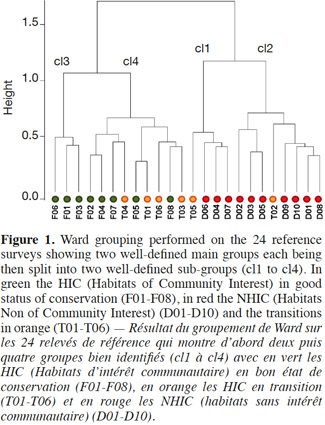
19Ordination confirms the partition into two groups on the first axis with HIC on the left (groups 3 and 4) and NHIC on the right (groups 1 and 2) (Figure 2).
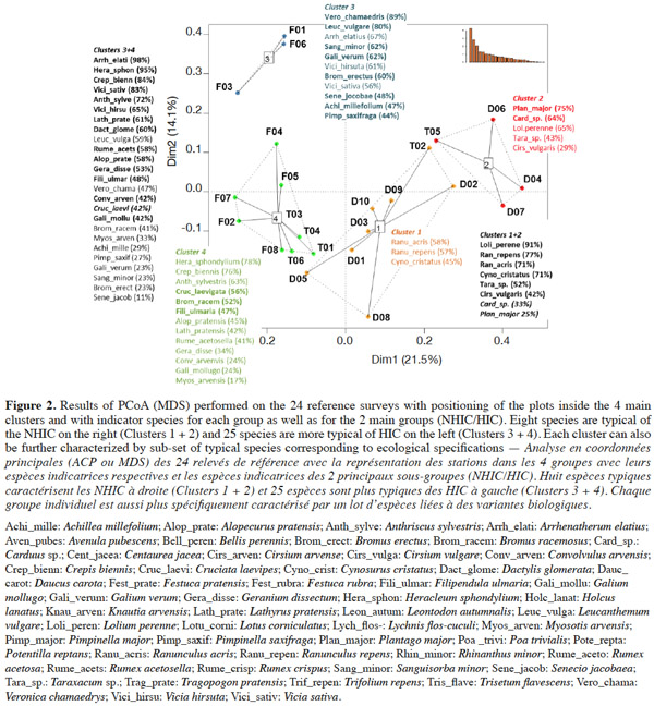
20A good match is observed between the reference typology (WalEUNIS and HIC codes), based on the frequency of the 14 characteristic species, and the overall phytosociological composition of hay meadows involving disturbance indicator species.
3.2. Variability in the diagnosis (presence/absence of a HIC)
21The table 1 shows that during the 93 surveys the four observers identified 71 (76%) HIC (38) and NHIC (33) correctly according to the reference observer’s opinion. They better identified the NHIC (33/40 = 83%) than the HIC (38/53 = 72%).
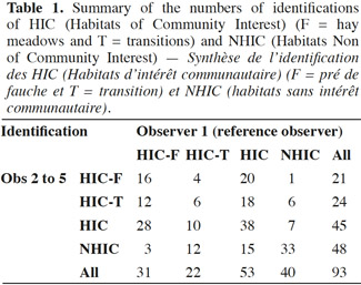
22The variability between the four observers is low because globally they identify 75% (OBS1), 71% (OBS2), 83% (OBS3) and 76% (OBS4) of the biotopes properly with a better proportion of HIC. Mismatches are more in the direction of under-detection of HIC (15 out of 93) than an overstatement of quality (7 out of 93).
23The same table shows that the transitions that are considered HIC present the most problems, with 12 identified HIC-T that are considered NHIC (55%) and only six plots considered HIC-T (27%) were correctly identified, according to first observer’s diagnosis. For HIC in good status (HIC-F), there is also a tendency to downgrade the diagnosis since only 16 (52%) plots of HIC-F are correctly identified and 12 (39%) were identified as transitions HIC-T. Overall, the rate of agreement with the reference observer was 59% if the difference between the HIC in good condition and transitions is taken into account.
24The variation between the four observers is more important since they correctly identified 54% (OBS1), 54% (OBS2), 71% (OBS3) and 57% (OBS4) of the biotopes.
25Overall, 15 out of 53 HIC (28%) and 7 out of 40 (18%) have not been identified as such.
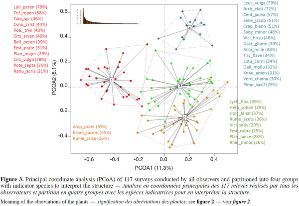
3.3. Variability of phytosociological surveys
26Multivariate analysis of 117 surveys shows (Figure 3) a strong opposition on the first axis of the principal coordinate analysis between, on one hand, the highly degraded plots (group 1) and, on the other hand, the other hay meadows, even the explained variability is relatively low (11%). The first group is characterized by a series of species typical of a marked deterioration. On the second axis, there is a gradient of increasing quality from the bottom to the top with surveys characterized by less and less indicator species of eutrophication (typical of group 2).
3.4. Sources of variability
27Non respect of determination criteria. As raw data from surveys conducted in the field are available, we can compare the diagnosis made by the four observers for the 22 surveys that do not correspond to the evaluation made by the first observer. For NHIC defined by observer 1, the other four observers identified 7 out of 40 as HIC (Table 1). In five of seven cases, records do not actually allow to characterize these habitats as HIC because even if the number of species is greater than or equal to three, the ratio of the total cover occupied by all indicator species standardized to 100% is well below 10%. In one case, the proportion of the cover of characteristic species before standardization to 100% actually exceeded 10%. The only case where the statement encoded justifies a HIC is actually questionable as an indicator species (Rhinanthus minor) is identified with a code Braun-Blanquet “2b” (20%), while other observers have not given that a code “+” (0.2%) or “1” (2.5%). This is probably an encoding error.
28For the HIC-F defined by observer 1, the other four observers identify only 3 of the 31 surveys as being NHIC (Table 1). In two of these three cases, the rules are respected because the statements made do not make it possible to characterize habitats HIC, and in the third case the cover is just above the threshold of 30% (product of the number of by species recovery). For the HIC-T defined by the observer 1, the other four observers identified 12 out of 22 surveys as being NHIC (Table 1). In 8 cases out of 12 raw data analysis confirms this diagnosis. In four other cases, the analysis of the survey should have easily lead to HIC qualification as the data meet the criteria, even before standardization to 100%. The distribution of the 22 differences between the four other observers with observer 1 is very balanced as it is between five and six for each of them.
29Overall, of the 22 issues identified, 10 surveys (NHIC 5, 1 HIC-F and 4 HIC-T) should have been classified quite easily by following the rules defined (minimum of three characteristic species and more than 10% of area occupied by these species). In the other 11 cases, data surveys lead to a qualification that does not match that of the first observer. Among the other 12 statements that could not be corrected by a strict application of the thresholds (see details in the “Supporting Information” section), 2 relate to situations where the number and the cover of characteristic species were already very close to the threshold before calibration to 100% cover and were re-classified as NHIC after calibration due to a significant overestimation (> 200%) of the total cover rate survey (F06_O5 and T06_O5). The other 10 cases are discussed in the two following paragraphs.
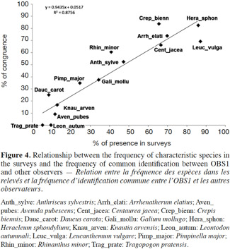
30Detection of characteristic species. Figure 4 shows the relationship between the relative frequency of species in 93 records of four observers and the relative frequency of common identification with the first observer. Clearly the more a species is common the more it is observed by different observers, suggesting a fairly random process. Some species such as Daucus carota, Rhinanthus minor, Crepis biennis are slightly better detected while Leontodon autumnalis or Leucanthemum vulgare are less, but the differences are small because the regression is largely significant (R2 = 87.5%).
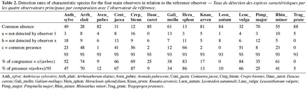
31Examination of the table 2 calls for the following comments. Several species are far more often detected by observer 1 than by other observers. Regarding L. autumnalis and C. biennis, it is possible that some observers confused these two species as they are very similar in the vegetative stage. This detection problem explains 6 of the 12 surveys that have not received the same diagnosis from the four observers with respect to the observer 1 and which are not due to improper application of rules (F08_O2, F08_O3, T04_O2, T04_O3, and T04_O4 T04_O5).
32Variability of cover estimates. Table 3 shows that overall, 55% of cover assessments are the same for observer 1 and the other four observers. Fairly clear differences were observed for some species that tend to be underestimated by the four observers (H. sphondylium and R. minor) or overestimated (A. sylvestris, C. jacea, C. biennis). In addition, a large variability in the estimated cover rate of A. elatius is observed since only 42% of the values are identical to those of the reference observer.
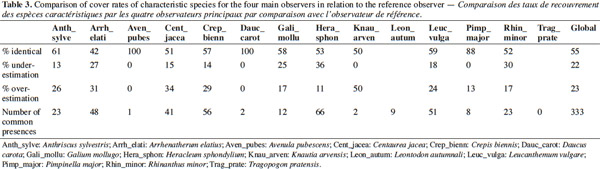
33However, with 60 under-estimations and 68 overestimations, 85% of the differences relate to differences of one-class variations and 59% of the 128 differences are due to variations between “+” and “1” Braun-Blanquet classes. This cover rate problem explains 4 of the 12 surveys that did not have the same diagnosis from the four observers with respect to the observer 1 and which are not due to improper application of rules (D01_O3, T05_O3, and T05_O5 T06_O2).
34Variability in sampling effort. A Poisson analysis (GLM) used to compare observers indicates (not presented here) that the reference observer saw more species on average than the other four observers, but this difference was significant only for observers 2 and 3 (significance level < 0.001). As regards the number of characteristic species, none of the differences is significant. The additional effort (approximately + 30% of the time spent on a plot) by the reference observer therefore is not manifested significantly for all parameters and compared with four other observers.
35But it emerged from several sequenced surveys (not presented here) that the standard error in assessing the theoretical number of characteristic species on a plot was lower when the survey was stopped after at least two consecutive periods of five minutes without detection of a new characteristic species.
4. Discussion
36As mentioned in the introduction, any study whose aims are to describe and to compare vegetation involving several observers is accompanied by a certain dose of variability that should be quantified before drawing any conclusions on the comparison of records (Hope-Simpson, 1940; Moore et al., 1970; Leps et al., 1992; Keating et al., 1998; Joint Nature Conservation Committee, 2004; Vittoz et al., 2007). The first step of this study was to validate the typology used for the 24 plots and further used as a reference when comparing the observers.
37A second step was to identify and quantify the sources of variability of the four main observers with respect to the first observer. Overall, the most typical HIC plots have been identified in 72% of cases and the most degraded ones (NHIC) in 83% compared with observer 1. Regarding transition habitats (HIC-T), only 27% are evaluated as such by the other four observers. Observers therefore tend not to overestimate the quality of a habitat as there are two times more underestimations of the quality of the habitats. The main causes of this variability are discussed below.
381. The examination of the consistency between the botanical surveys and the habitat code given by the observers has shown that they have regularly not respected the criteria when classifying the habitat as a HIC or a HNIC in plots of transition habitat (discordant diagnoses in 22 surveys whereas ten of them should have been diagnosed correctly if the criteria had been respected).
39Two cases of the 12 surveys relate to cases when the values of the parameters (number and cover rate of characteristic species) were very close to the theoretical thresholds and were declassified after standardization at 100% due to an excessive overestimation of the total cover rate (> 200%). This important source of discrepancy between the observers could easily be solved (see below).
402. Another source of variability is the detectability of the characteristic species. This problem has affected 6 of the 12 cases of discordance with the diagnosis of the first observer not attributable to poor respect of the rules. Generally the more a species was common in 24 plots, the more it was detected and the more the species was rare, the more it escapes the observer. Vittoz et al. (2007) also showed that species whose cover rate is less than 0.1% in small plots (40 m2) are frequently undetected by observers. However, other factors are also involved linked to the very characteristics of the plant. Leucanthemum vulgare was significantly less detected by the four observers than by the reference observer, probably because the basal leaves are more difficult to detect in the canopy of a hay meadow when the plant is not flowering. Similarly, Tragopogon pratensis is often present in the form of isolated linear leaves that can easily go unnoticed during a survey.
413. Another important source of variability is the assessment of the cover rate especially of grasses. Overall, 55% of cover assessments are identical for observer 1 and the other four observers.
42Even if in the remaining 45%, 85% of the differences concern only variations of a single Braun-Blanquet class and 59% concern variations of very low cover classes (“+” and “1”), these differences can have a significant impact on more abundant characteristic species such as A. elatius, C. biennis, C. jacea, H. sphondylium, L. vulgare and to a lesser extent R. minor. However, even if it is possible to reduce the magnitude of this factor, for example through targeted training (see below), a certain amount of variability is inevitable and should be kept in mind when comparing records with the aim at detecting possible changes in the grassland plot. A similar study conducted by Leps et al. (1992) showed that only 57.5% of the species were recorded with the same level of abundance by different experts, 39.5% of the species were recorded with a difference of one degree in the scale of Braun-Blanquet and 3% with more than one degree. Traxler (1998) found also that 52% of the species were in the same class of abundance. Hope-Simpson (1940) had obtained comparable figures with a single observer doing repeated surveys on a series of plots and Vittoz et al. (2007) obtained coefficients of variation between eight observers from more than 50% on plots measuring 40 m2.
434. A last important factor is due to the prospection effort. Several sequenced surveys suggest that when an observer deliberately delivers a greater prospection effort than “in routine”, this produces a slight positive effect (in terms of total species richness) for two of the four other observers, but has no significant effect as regards the number of characteristic species.
44Other sources of variability have been identified and even if their impact is likely to be lower, they must also be taken into account in order to improve the quality of surveys: the size of the plot, the natural fluctuations in abundancy between years (Swaine et al., 1980; Smith et al., 1985) and errors made during field transcription and during encoding (in our study 34 duplicates were detected for a total of 7,431 species encoded).
5. Solutions and corrective measures
45In a logical sequence of improvement of the surveys from the protocole to the field survey itself, we suggest the following solutions and corrective measures:
461. To reduce the variability of botanical data collected (characteristic species not of falsely detected, variable cover rate), new field training should be provided to experts in charge of the surveys targeting the evaluation of cover rate assessment (in particular for grasses as well as more difficult species to identify correctly like the yellow Asteraceae). However, it is necessary to keep in mind that even if these problems can be improved through inter-calibration between experts, it is well known that this factor is impossible to control completely (Leps et al., 1992). It therefore seems reasonable to consider in the future that there is a true degradation of a HIC (6,510) only if there is a decrease in the cover rate of all characteristic species by a minimum of 10%. This figure is to be compared with the recommendations of the Joint Nature Conservation Committee (2004) which declares a meadow as “degraded” between two statements when the species characteristic of degradation have collectively increased by at least 10% of the global cover.
472. Since it is very likely that some of the variation in the assessments of the cover rate come from an incomplete running through some plots (the largest plots are the most vulnerable to this type of error), it should be advisable to divide virtually plots over 1 ha (indicative figure) and make two or more separate surveys specifying the respective areas inventoried.
483. Regarding the cases when there was no consistency between the botanical survey and the WalEUNIS code given by an observer, it appears that a quick calculation in the field when taking notes (calculating the number of characteristic species and their cover rate) would greatly reduce the number of cases where the observer gives a Waleunis/EUR_15 code that does not match his botanical record. This quick calculation is also suggested to avoid the tendency to overestimate the total cover rates leading in some cases to a downgraded diagnosis. A quick check of the total coverage noted at the time of the survey would make sure that this sum is between 100 and 150% and if possible does not exceed 120%, which in most cases, corresponds more to reality.
494. Another lesson learned from these tests is that the survey effort was often inadequate. Even if detecting and identifying all species present on a spot station is illusory and unproductive (Nilsson et al., 1985; Keating et al., 1998), it is still essential to compare the numbers of characteristic species on a similar basis using a reasonable prospection effort. We evaluated that a survey of 30 min allows in most cases for 95% of the characteristic species in plots of reasonable size (about 1 ha). An important instruction to give to all experts would be to not stop a survey until no new characteristic species has been detected for at least two consecutive periods of 5 min, which corresponds to a “plateau” of three points on the curve theoretical. In this respect Klimes et al. (2001) estimated that a single period of at least 5 min without detection of new species during surveys conducted on much smaller surfaces was sufficient (0.25 to 4 m2). It must be stressed however that precautions must be taken when interpreting the theoretical values generated by these theoretical models because other factors may influence these estimates, such as the level of expertise of each observer, species detectability in relation to the stage of vegetation, and the size and heterogeneity of the plot (Kéry et al., 2008).
505. To avoid encoding “duplicates” an automatic check has been programmed (by Yvan Barbier) in the database that signals to the encoder a possible duplicate.
51Finally, as regards the monitoring (every six years), we recommend, based on what has been exposed above:
52– to work as much as possible with the same group of observers (whose potential biases have been assessed);
53– when surveying plots, to take along old records, assuming that they can be considered almost exhaustive, in order to detect an actual potential decline in the quality of the plot (Leps et al., 1992).
54Acknowledgements
55We would like to thank Éric Fauconnier, Étienne Peiffer and Séverin Pierret for their help during the field campaign. We are also grateful to Mr Quentin Groom, researcher, for his conscientious reading of the English version.
Bibliographie
Bottin G., Étienne M., Verté P. & Mahy G., 2005. Methodology for the elaboration of Natura 2000 sites designation acts in Walloon region (Belgium): calcareous grasslands in the Lesse and Lomme area. Biotechnol. Agron. Soc. Environ., 9, 93-99.
Davies C.E. & Moss D., 2002. EUNIS habitat classification, February 2002. Paris: European Topic Centre on Nature Protection and Biodiversity.
Dufrêne M. & Legendre P., 1997. Species assemblages and indicator species: the need for a flexible asymmetrical approach. Ecol. Monogr., 67, 345-366.
Dufrêne M. & Delescaille L.-M., eds, 2005. La typologie WalEUNIS des biotopes wallons, version 1.0., http://biodiversite.wallonie.be/fr/dufrene-m-delescaille-l-m-eds-2005-la-typologie-waleunis-des-biotopes-wallons-version-1-0-spw-dgarne-spw-base-de-donnees.html?IDD=167776631&IDC=3046, (21.04.15).
Dufrêne M., Delescaille L.-M. & Derochette L., 2013. La méthodologie de cartographie, d’inventaire et d’évaluation des états de conservation dans les sites Natura 2000 en Région wallonne. In: Born C.-H. & Haumont F., eds. Actualités du droit rural : vers une gestion plus durable des espaces ruraux ? Louvain-la-Neuve, Belgique : Larcier, 43-55.
European Commission, 2013. Interpretation manual of European union habitats - Eur28. European Commission, DG Environment, Nature & Biodiversity, http://ec.europa.eu/environment/nature/legislation/habitatsdirective/docs/Int_Manual_EU28.pdf, (21.04.15).
Halford M. & Peeters A., 2006. Appui scientifique à la mise en œuvre du Réseau Natura 2000 en Région wallonne. Finalisation de la typologie WalEUNIS, synthèse des états de conservation, critères de restauration et mesures de gestion pour les prairies semi-naturelles, les mégaphorbiaies et les ourlets forestiers. Louvain-la-Neuve, Belgique : Unité d'Écologie des Prairies, UCL.
Hope-Simpson J.F., 1940. On the errors in the ordinary use of subjective frequency estimations in grassland. J. Ecol., 28(1), 193-209.
Joint Nature Conservation Committee, 2004. Common standards monitoring guidance for lowland grassland habitats, http://jncc.defra.gov.uk/PDF/CSM_lowland_grassland.pdf, (21.04.15).
Keating K.A., Quinn J.F., Ivie M.A. & Ivie L.L., 1998. Estimating the effectiveness of further sampling in species inventories. Ecol. Appl., 8(4), 1239-1249.
Kéry M. & Royle J.A., 2008. Hierarchical Bayes estimation of species richness and occupancy in spatially replicated surveys. J. Appl. Ecol., 45, 589-598.
Kirby K.J. et al., 1986. Seasonal and observer differences in vascular plant records from British woodlands. J. Ecol., 74, 123-131.
Klimes L. et al., 2001. Scale-dependent biases in species counts in a grassland. J. Veg. Sci., 12, 699-704.
Lambinon J. & Verloove F., 2012. Nouvelle flore de la Belgique, du Grand-Duché de Luxembourg, du Nord de la France et des régions voisines (Ptéridophytes et Spermatophytes). Meise, Belgique : Édition du Jardin botanique national de Belgique.
Legast M., Bottin G., Étienne M. & Mahy G., 2006. Appui scientifique à la mise en œuvre du réseau Natura 2000 en Wallonie : finalisation de la typologie WalEUNIS et synthèse de états de conservation, critères de restauration et mesures de gestion pour les habitats semi-naturels ouverts. Rapport final, http://orbi.ulg.ac.be/handle/2268/12422, (21.04.15).
Legendre P. & Legendre L., 2012. Clear and comprehensive approach to the numerical methods that are successfully used for analysing ecological data. Numerical ecology. 3rd ed. Elsevier.
Leps J. & Hadincova V., 1992. How reliable are our vegetation analyses? J. Veg. Sci., 3, 119-124.
Moore J.J., Fitzsimons S.J.P., Lambe E. & White J., 1970. A comparison and evaluation of some phytosociological techniques. Vegetatio, 20(1-4), 1-20.
Nilsson I.N. & Nilsson S.G., 1985. Experimental estimates of census efficiency and pseudoturnover on islands: error trend and between-observer variation when recording vascular plants. J. Ecol., 73, 65-70.
Oksanen J., 2013. Multivariate analysis of ecological communities in R: vegan tutorial, http://cc.oulu.fi/~jarioksa/opetus/metodi/vegantutor.pdf, (21.04.15).
Scott W.A. & Hallam C.J., 2002. Assessing species misidentifications rates through quality assurance of vegetation monitoring. Plant Ecol., 165, 101-115.
Smith I.R., Wells D.A. & Welsh P., 1985. Botanical survey and monitoring methods for grasslands. Grassland Habitat Network Handbook Number 1. Peterborough, UK: Nature Conservancy Council.
Swaine M.D. & Greig-Smith P., 1980. An application of principal components analysis to vegetation change in permanent plots. J. Ecol., 68, 33-41.
Traxler A., 1998. Handbuch des Vegetationsökologischen monitorings. Methoden, Praxis, angewandte Projekte. Teil A: Methoden. Monographien 89 A. Wien: Umweltbundesamt.
Vittoz P. & Guisan A., 2007. How reliable is the monitoring of permanent vegetation plots? A test with multiple observers. J. Veg. Sci., 18, 413-422.