

- Accueil
- Volume 89 - Année 2020
- Articles
- Quantifying the effects of spatial patterns of green spaces on urban climate and urban heat island in a semi-arid climate


Visualisation(s): 2955 (15 ULiège)
Téléchargement(s): 16 (0 ULiège)

Quantifying the effects of spatial patterns of green spaces on urban climate and urban heat island in a semi-arid climate

Document(s) associé(s)
Version PDF originaleAbstract
Green spaces in urban areas have a positive effect on the urban climate and microclimate. They help regulate the urban climate and mitigate the urban heat island (UHI) by creating a cooling effect through shade and evapotranspiration. In addition, they release oxygen, absorb carbon dioxide, generate shade, as well as energy usage and pollution emissions. The aim of this study is to assess the impact of spatiotemporal changes in green cover on the urban climate to mitigate the urban heat island (UHI). This is achieved through analyzing their effects on the land surface temperature (LST) due to the change in the spatial configuration of this green cover in the period between 1990 and 2019 in Constantine city. To materialize this effect, Google Earth Pro images, Landsat 5TM and Landsat 8 OLI/TIRS images of multiple years were acquired, processed and analyzed to generate land use maps (LU/LC), the normalized difference vegetation index (NDVI) maps. Those maps were used in order to estimate land surface temperature LST, the green cooling island (GCI) and the urban cooling island (UCI) of vegetation. Many landscape metrics (PLAND, CA, PD, NP, LPI, LSI, MPS, AI, PR, and SHAPE_MN) were chosen for the study at the class and landscape level to analyze the relationship between spatial patterns of vegetation and spatial distribution of LST through the SPSS 26 software.
Our results showed that there is a negative relationship between NDVI and LST during the study period. Thus, the increase in NDVI values caused a decrease in LST values. Dense green space with the highest values of NDVI had the highest cooling effect. Therefore, our study confirmed that the type, density, size and the shape of vegetation are important factors in determining its cooling effect. The obtained results showed also that a simple, homogeneous and aggregated green landscape is more effective. The large dominant green patch has the highest impact on LST distribution leading to fragmented green patches with complicated shapes which led to an increase in LST.
Table des matières
1. Introduction
1The study of the urban heat island effect (UHI) is becoming more and more serious with the increase in the built-up areas at the expense of green surfaces which are the origin of global climatic change (Parker, 2010). Today, more than 50% of the world's population lives in cities. This percentage is rising, especially in developed countries (United Nations, 2011). This rapid increase in population generates an accelerated process of urbanization which leads to a severe decrease in green spaces and a rapid increase in the built-up area (Guo et al., 2012, Landsberg, 1981). This transformation makes the city center warmer than its surroundings. One important effect of this phenomenon is called the urban heat island (UHI). The term “urban heat island” refers to an urban area where air and surface temperature is higher than those in rural areas. Constructions, asphalt and concrete absorb solar radiation and emit longwave radiation in the form of waste heat which contributes to the warming of the urban heat island (Miller et al., 2015). The built-up areas and the impervious surfaces (Tar, concrete, various building materials) are characterized by low albedo, high impermeability and thermal properties which are favorable for energy storage and releasing heat. Therefore, the transformation of the natural and green landscapes into built-up areas and impervious surfaces makes this urban area warmer than the surrounding areas. This is called the urban heat island (UHI) which is identified as the meteorological impacts of dense urbanization.
2The phenomenon of urban heat island causes real heat zones due to human activity and dense urbanization which negatively affect the human thermal comfort in the urban area and increase the risks of pollution and many other problems (Maheng et al., 2018).
3Trees and plants are important elements for earth system. They help to regulate the urban climate and mitigate the Urban Heat Island by creating a cooling effect, giving off oxygen, absorbing carbon dioxide, minimizing and intercepting the sun's rays, generating the shade and absorbing the fluxes of radiation. (Kong et al., 2014, Taha et al., 1988, Oliveira et al., 2011). Furthermore, the vegetation type and density, green space size and shape, and trees shaded areas are all important parameters in determining the cooling effect (Gherraz et al., 2018 , Hanafi & Alkama, 2017 , Giridharan et al., 2008). Green surfaces may effectively contribute to the reduction of higher temperatures which are caused by UHI effects by keeping its temperature low. They also extend the cooling effect beyond the boundary of these surfaces. Therefore, planting vegetation in urban areas and the good choice of its type and size in particular are the main strategies which are employed to regulate the urban climate and create cooler urban spaces (Tan & Li, 2013). Thus, changing the plants and trees around us can affect our health, our environment, and our comfort. Improvements in air quality due to vegetation certainly have a positive impact on physical health as it is beneficial in reducing respiratory illnesses. The link between man and nature is important for daily pleasure, productivity at work and general mental health (Sorensen. et al., 1997). For these reasons, the subject of vegetation’s life becomes a question of extreme importance for scientists (Wu, 2014).
4Several studies have investigated the impact of parks and green spaces on the urban microclimate (Boudjelal & Bourbia, 2017, Qiu et al., 2017, Zhang, 2017, Chun & Guldmann, 2018). They have deduced that the reduction in temperature in a green urban environment can reach 4 °C (Gherraz et al., 2018). However, many studies (Cohen et al., 2012) have predicted that urban green spaces could be warmer than the surrounding built-up area and could worsen unpleasant microclimatic conditions. Chatzidimitriou (2006) revealed the importance of shading paved surfaces. Shaded surfaces have 21% lower temperatures than air temperature. Also, they are 40% cooler than the same surfaces exposed to direct sunlight (Chatzidimitriou et al., 2006, Shahidan et al., 2007).
5A review of the state of the art in the field shows that urban green spaces can make an urban cool island effect (UCI). This urban cool island effect is created by the shading or perspiration effects of urban trees which are affected by green spaces and water bodies. This effect can be assessed by the LST difference between green spaces and their surroundings (Hongyu et al., 2017). Recently, these studies have focused on the role of urban vegetation in the regulation of LST. They have proved that the LST could have been decreased by increasing the area of the green cover and the fraction of the water spaces (Chen & Wong, 2006, Hamada & Ohta, 2010). According to Kong (2014), urban green spaces can also generate a localized cooling effect (urban cool island UCI) which is an effective way to mitigate the UHI effect and provide a comfortable outdoor environment. It can be determined by a number of many important factors such as the type and density of vegetation, the size and shape of green spaces and the shade area of trees. For example, trees are more effective than bushes which in turn are more effective than grass (Kong et al., 2014, Cao et al., 2010).
6Landscape metrics have been effectively applied in different areas of environmental research, including management and assessment of water resources, delimitation of protected areas, assessment of the environmental impact of the urban growth mechanism and landscape rehabilitation plans (McGarigal et al., 2005). In addition, some research studies have investigated the relationship between the spatial characteristics of land use in particular green cover and built-up areas on the LST (Cao et al., 2010, Zhang et al., 2009, Weng et al., 2007, Zhou et al., 2011, Weng et al., 2007, Liu & Weng, 2009). These studies have indicated that landscape parameters retain significant potential for exploring the LST spatial model.
7The aim of this study is to evaluate the spatiotemporal changes of vegetation as well as its impact on the microclimate to mitigate the urban heat island. The research seeks to estimate the intensity of the green cool island (GCI) and the urban cool island (UCI) of vegetation in Constantine city. It also studies how and to what extent the land surface temperature (LST) is affected by the spatial configuration of the green landscape. In order to materialize this effect, from one hand the remote sensing technique was used. From the other hand we have used the landscape ecology theory which is the study of spatial variation in landscapes at different scales. It is used to assess the impact of the composition and spatial configuration of the vegetation cover on the distribution of land surface temperature LST using the landscape metrics.
2. Materials and methods
2.1 Study area
8The study was conducted in the Constantine city in Algeria. It is located approximately 431 km away from the capital Algiers. It is 245 km away from the Algerian-Tunisian borders. It is also 89 km away from Skikda to the north and 235 km away from Biskra to the south. Its position gives it a strategic location to consist a link between the cities of the south and the coastal cities. It is located 36° 17' in latitude and 6°37' in longitude (Figure 1). Moreover, it is located in the center of a pinch between the mountains (Djebel Ouahch and Djebel Chettaba) on a majestic rock located on both sides of Oued Rhumel. The site is marked by the juxtaposition of two hills (El Mansourah and Ain El Bey) (Figure 2)
9In addition to that, the city is located in a region between the Sahara in the south with a continental climate and the influence of the Mediterranean climate in the north which is characterized by irregular rainfall and a long period of summer drought. So the climate of the city is a cool semi-arid which is characterized by two distinct periods: a wet and cold winter with 197 days and a dry and hot summer with 133 days.
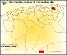
Figure 1: Geographical situation of Constantine city
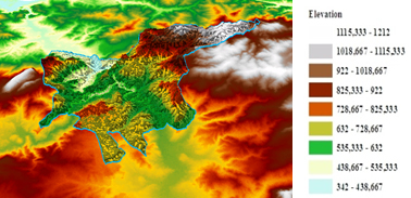
Figure 2: 3D topographic map of Constantine city through ArcScene 10.5
2.2. Data processing & analysis
10Landsat imagery is the main data source for classification and analysis. Landsat imagery data include Landsat Thematic Mapper (TM) and OLI/TIRS geo-referenced scenes for the years 1990, 2000, 2005, 2010, 2015 and 2019 respectively in the same season (the dry season) exactly in June (the use of 2 images of Landsat is because of the availability of TM images before the creation of OLI / TIRS in 2013). These datasets were acquired from the National Aeronautics and Space Administration (NASA) through their USGS (Earth Explorer) Data Gateway Database. The pre-processing and the processing were performed using ArcMap 10.5 software, FRAGSTATS 4.2.1, SAGA and SPSS 26. The details of Landsat images were incorporated in the study given in Table 1.
Table 1: Summery of Remote Sensing data used in this study
|
Satellite |
Date |
Time |
Sun azimuth |
Sun elevation |
Cloudcover |
WRS path |
|
Landsat 5TM |
1990-06-24 |
09:27:30 |
106.1049385 |
60.0376830 |
0.00 |
193 |
|
2000-06-03 |
09:43:25 |
113.5118685 |
63.2847977 |
0.00 |
193 |
|
|
2005-06-08 |
10:01:00 |
116.0255042 |
65.5377627 |
1.00 |
194 |
|
|
2010-06-22 |
10:04:06 |
115.0124398 |
65.9116536 |
0.00 |
194 |
|
|
Landsat 8 OLI |
2015-06-29 |
10:06:42 |
118.0622757 |
67.1399442 |
0.00 |
193 |
|
2019-06-24 |
10:07:12 |
118.2548474 |
67.5160376 |
0.01 |
193 |
The methodological process was carried out through the following steps (Figure 3).
The first step was to generate Land use maps through the use of supervised classification. This classification is firstly consisted of choosing training plots (ROI) which are pixels grouped according to the characteristics of a given land occupation based on the knowledge of the land use and on the spectral signature. Then, the Maximum Likelihood Classification algorithm was used to classify the images. It estimates the means and the variance from the image training sites. This consisted of choosing the pixels which corresponded to the means and variance values. This algorithm offered a good generalization capacity.
The second step includes estimating the changes in NDVI index and land surface temperature LST. It also investigates the relationship between those two indices Via SAGA 7.4.0. It calculates the green cool islands GCI and the urban cool Island UCI of vegetation.
2.2.1 Normalized Difference Vegetation Index NDVI
It was the most used vegetation index; it was calculated from the visible and near-infrared light reflected by vegetation. The healthy (with a good evapotranspiration processes) vegetation absorbed most of the visible light that hits it, and reflected a large portion of the
.processes) reflected more visible light and less near-infrared light (Weier & Herring, 2000).
The NDVI was defined by this formula:
|
NDVI= ρNir - ρred / ρNir + ρred |
(1) |
Where: ρNir = reflectance of objects for near-infrared;
ρred = reflectance of objects for visible red band.
11Calculations of NDVI result in a number that ranges from (-1) to (+1). Whereas, the extreme negative values represent water. Values around zero represent bare soil and values close to +1 (0.8 - 0.9) indicates very dense vegetation. In order to calculate the NDVI index we need to use the Band 3 (Red Band) and Band 4 (NIR Band) of Landsat 5TM and band 4 (Red Band) and the band 5 (NIR Band) of Landsat8 OLI/TIRS. The NDVI index offers the possibility to analyze the change in vegetation cover during the period of the study. It will be correlated with the LST to analyze the impact of vegetation on the surface temperature.
2.2.2 Land Surface Temperature LST
12LST plays an important role in the physics of land surface as it is involved in the processes of energy and water exchange with the atmosphere. Land surface temperature of the study area was retrieved from the thermal infrared band of Landsat images. The approach used in this study for LST retrieval is a simple single-channel algorithm which can be employed for coarse resolution images. The method incorporates atmospheric profile values and emissivity obtained from NDVI, thereby improving the accuracy of the extraction. Since the time period considered for the study is from 1990 to 2019 and the used dataset is Landsat 5TM and 8 OLI/TIRS data, an LST extraction method which can be applied to sensors with single thermal band data was adapted for the study. In order to estimate land surface temperature LST, we have calculated many other indices such as (Boudjellal & Bourbia, 2018):
13- The Atmosphere Reflectance: OLI and TIRS band data could be converted to TOA spectral radiance rescaling factors provided in metadata file:
|
Lλ' = Mp x Qcal + Ap |
(2) |
14Where: Lλ' =TOA Planetary Spectral Reflectance, without correction for solar angle;
15Mp = Reflectance multiplicative scaling factor for the band;
Qcal = L1 pixel value in DN (Digital Numbers)
16Ap = Reflectance additive scaling factor for the band.
17- Atmosphere Brightness Temperature: TIRS band data can be converted from spectral radiance to top of atmosphere brightness temperature using the thermal constants in the metadata file:
|
TB= K2/ ln (K1/+ Lλ'+ 1) |
(3) |
18Where: TB = TOA Brightness Temperature, in Kelvin;
19Lλ = Spectral radiance (Watts/(m2 * srad * μm))
20K1 = Thermal conversion constant for the band (K1_CONSTANT_BAND_n from the metadata)
21K2 = Thermal conversion constant for the band (K2_CONSTANT_BAND_n from the metadata).
22- Estimation of Fractional Vegetation Cover (FVC) for an image using NDVI:
|
Pv= [(NDVI – NDVImin)/ (NDVI – NDVImin)] 2 |
(4) |
23- Estimation of Land Surface Emissivity (LSE):
|
ɛ= 0.004 x Pv + 0.986 |
(5) |
24- Estimation of Land Surface Temperature (LST):
|
LST= TB/ 1+ (Lλ'+TB/P) x ln(ɛ) |
(6) |
2.2.3 Quantifying the Green Cool Island effect GCI
25The cooling effect of green spaces has been widely studied. Jusuf et al., (2007) have studied the distribution of air temperature in Singapore using remote sensing data and mobile survey data. Temperature has been found to be significantly correlated with land characteristics. It decreased as the density of greenery increased (Jusuf et al., 2007). The effect of GCI was evaluated by the LST temperature difference between green spaces and their environment.
26It was calculated with this formula (Boudjellal & Bourbia, 2018):
|
GCI = ΔLST = LSTU – LSTO |
(7) |
27Where LSTo represents the average LST value inside the vegetation class, and LSTu represents the average of LST in the urban area.
2.2.4 Quantifying the Urban Cool Island effect UCI
28The UCI generally refered to the phenomenon when green spaces had a lower temperature than that of the surrounding areas. Studies relating to the UCI of air used the atmospheric temperature which is acquired from fixed weather stations or mobile equipment. Observations related to atmospheric temperature have demonstrated that the size and shape of vegetation patches; just as tree species; are important factors in influencing the cooling effects (Fintikakis, 2011). These observations have shown that urban green spaces were 1°C to 7 °C cooler than the surroundings. On average, large parks were generally cooler than smaller ones because urban cool islands (UCIs) in parks were more related to the characteristics of the parks (Chang, 2015). This index was calculated using the following formula:
|
UCI= ∆T = Ti−¯T (∆T ≤ 0) |
(8) |
29Where (¯T) is the mean LST of the study area and Ti is the temperature in each pixel.
30Our study focuses on understanding what or which spatial characteristics of green patches were likely to influence the spatial variability of LST. Thus, the third step is to estimate the landscape metrics (Table 2) and investigate the relationship between the spatial configuration of the green cover and the spatial distribution of LST. Our choice of landscape metrics was based on the metrics often used to analyze vegetation. Some were selected according to the size. Some were selected according to the shape complexity. Others were chosen according to the aggregation and fragmentation. To materialize this, the FRAGSTAT software which allows us to calculate the landscape metrics at two class-level spatial metrics (at landscape level and class level) was used. Finally, the SPSS 26 software was used to investigate the relationship between landscape metrics and LST.
Table 2: Landscape metrics used in this study
|
Level |
Description |
Unit |
Range |
||
|
CA |
Class/ landscape |
The total class area |
Hectares |
CA > 0, No limit |
|
|
PD |
Class/ landscape |
The number of patches per unit area |
N/100 ha |
PD > 0 |
|
|
PLAND |
Class/ landscape |
The proportion of total area occupied by a particular patch type; a measure of landscape composition and dominance of patch types |
% |
0 < PLAND < 100 |
|
|
NP |
Class/ landscape |
The number of patches of the corresponding patch type/landscape |
None |
NP ≥ 1, No limit |
|
|
LPI |
Class/ landscape |
The area (m2) of the largest patch of the corresponding patch type divided by total landscape area (m2), multiplied by 100 (to convert to a percentage) |
% |
0 < LPI < 100 |
|
|
LSI |
Class/ landscape |
A modified perimeter area ratio, a measure of overall shape complexity of patches of a given type |
None |
LSI≥1, No limit |
|
|
MPS |
Class |
The area occupied by a particular patch type divided by the number of patches of that type |
Hectares |
MPS> 0 No limit |
|
|
AI |
Class/ landscape |
AI equals the number of like adjacencies involving the corresponding class, divided by the maximum possible number of like adjacencies involving the corresponding class, which is achieved when the class is maximally clumped into a single, compact patch; multiplied by 100 (to convert to a percentage). |
% |
0 ≤ AI ≤ 100 |
|
|
Shape MN |
Class |
Mean value of shape index of a particular patch type |
None |
≥ 1, No limit |
|
|
PR |
Landscape |
The number of patch types in the landscape; a measure of diversity of patch types |
None |
PR≥1, No limit |
|
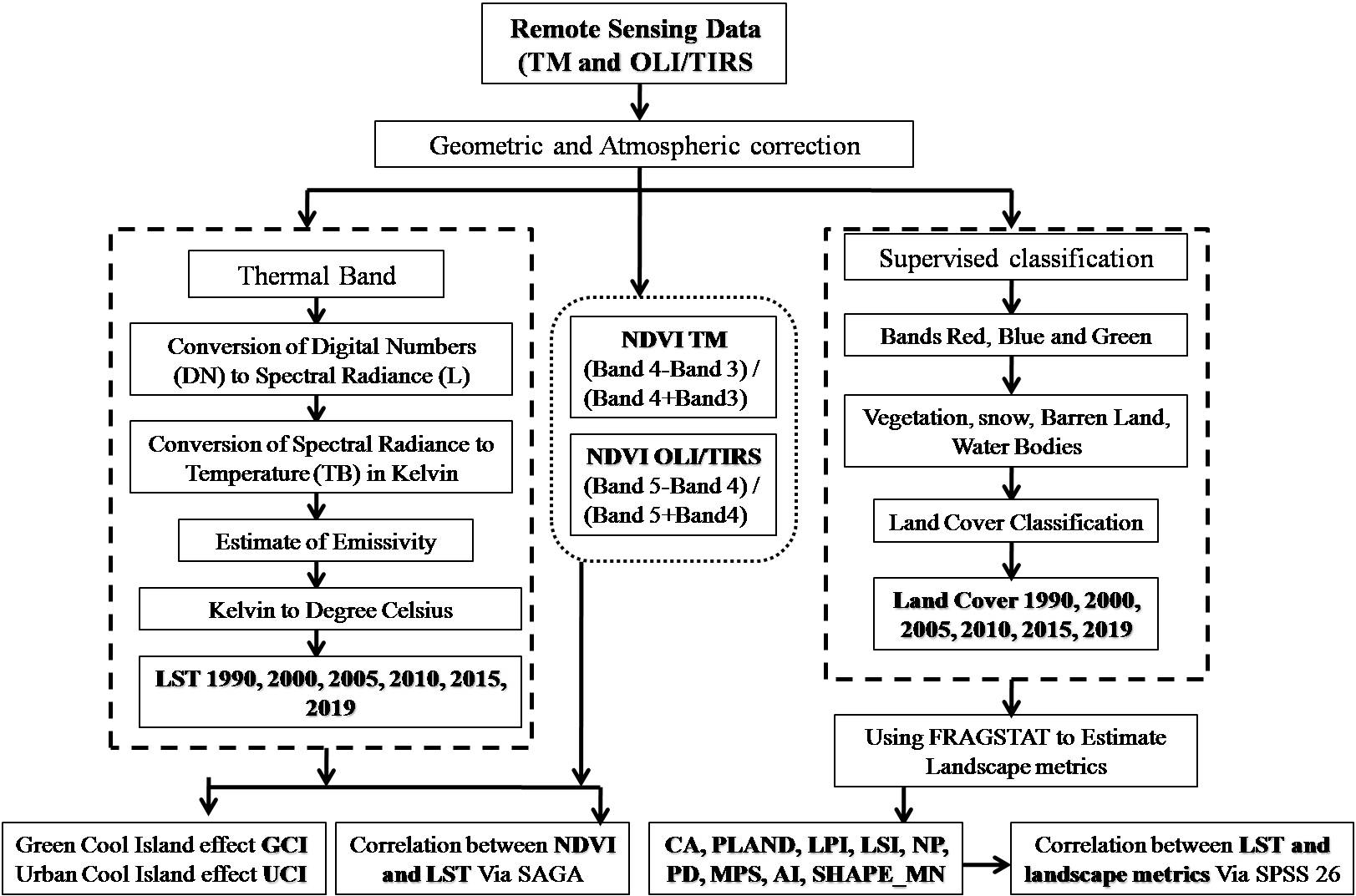
Figure 3: Flowchart of research methodology incorporated in the study.
3. Results
3.1 Preparation of Land use/ Land Cover LU/LC map
31
32The green cover species in Constantine city varied between forests, trees, high-stemmed plants and ornamental plants. Land use was divided as follow:
33- High vegetation: basically covered by trees and shrubs; grass land
34- Low vegetation: basically covered by lawn, large dry crop and irrigated crop;
35- The urban area: residential and industrial zones, there was no water body in this city (Fig 4).
36The land use maps showed the evolution of the urbanized area during the study period in several directions. Knowing that during the second Quadrennial Plan 1974–1977 (a short-term development plan generally of 4 to 5 years, it provides for the establishment of the infrastructure and equipments necessary for the development of the economy, agriculture and housing), the authorities gave importance to housing and urban planning sector in order to take charge of the housing crisis which was at its peak. Through this plan, an urban policy integrated into national development has been implemented. This was materialized by the creation of major housing construction programs in the form of Z.H.U.N in the east and north of Constantine, such as the Ziaidia, Daksi, August 20 neighborhood and July 05 neighborhood. Due to a lack of surfaces to be urbanized, Constantine's growth during the 1980s took place outside its urban perimeter with the creation of the ZHUN of Békira in the North, Zouaghi in the South and Boussouf in the West. Furthermore, individual housing developments were located on these same sites. The urban expansion of this city continued without planning along the communication axes.
37This urban growth results in green surface reduction. Constantine city comprises of 150 hectares of urban forests after independence, whereas; currently it only comprises of 50 hectares. The forest of El Mansorah used to comprise of 61 hectares, currently it occupies only 7.11 hectares. The forest of Sidi Mebrouk sector used to occupy an area of 20 hectares, currently it occupies only 13 hectares. Other forests such as “Sidi Djellis forest which used to occupy 32 hectares, and the forest of Sidi M'cid which used to occupy 8 hectares” have completely disappeared (Ali Khoudja, 2011).
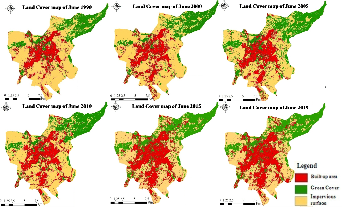
Figure 4: Land use maps, June 1990, 2000, 2005, 2010, 2015 and 2019 respectively
3.2 Production of Normalized Difference Vegetation Index NDVI
38The NDVI values extracted from the map (Figures 5) are given in Table 3. The results indicated an important difference during the study period. The green cover varied from one year to another. We have recorded negative values which represent bare soil and impervious surfaces in 1990, 2000 and 2010. The positive values between 0 and 0.3 represent low vegetation which occupied the majority of the studied area. Values which were more than 0.3 represent dense vegetation or forests. Those maximum values change from one year to another because of the severity of the cold season (frost) and the volume of precipitation or fires in the dry season. The maps also showed a considerable increase of green cover (the area occupied by vegetation) in recent years. This increase is due to the policy which is launched by the authorities through the creation of several green spaces such as Bardo Park, the establishment of alignment trees and green spaces in residential areas. We have recorded lower NDVI values in recent years due to fires in different forests which influence the green cover quality.
Table 3: NDVI index values in the period 1990-2019
|
June 1990 |
June 2000 |
June 2005 |
June 2010 |
June 2015 |
June 2019 |
|
|
NDVI min |
-0.354 |
-0.511 |
-0.346 |
-0.361 |
-0.152 |
-0.067 |
|
NDVI mean |
0.082 |
0.114 |
0.165 |
0.148 |
0.169 |
0.187 |
|
NDVI max |
0.575 |
0.728 |
0.622 |
0.712 |
0.583 |
0.526 |
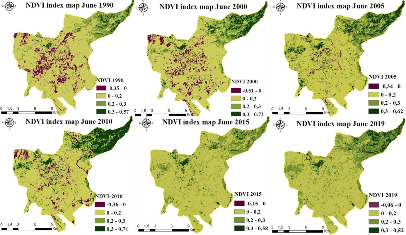
Figure 5: NDVI map of June 1990, 2000, 2005, 2010, 2015 and 2019 respectively
3.3 Land surface temperature LST retrieval
39The LST values extracted from the map (Figures 6) are given in Table 3. The maps showed that the LST values varied between 20.1 °C and 44.3 °C during the study period. The maximum values were registered in 1990 with the minimum values of NDVI, while the minimum values are registered in 2010 with the maximum values of NDVI. Temperature peaks were recorded at the level of impervious surfaces and bare land, whereas; the lowest values were recorded in dense vegetation and forests. In the built-up area we have recorded mean values. A slight difference was recorded in NDVI and LST of 2010 and 2015. This difference is due to the harvest period of cultivated lands intended for the cultivation of wheat in this region.
40
41
Table 4: LST values in the period 1990-2019
42
|
June 1990 |
June 2000 |
June 2005 |
June 2010 |
June 2015 |
June 2019 |
|
|
LST min |
26.9°C |
23.2°C |
23.2°C |
20.15°C |
23.29°C |
20.2°C |
|
LST mean |
36°C |
34.4°C |
32.8°C |
31.16°C |
35°C |
32.02°C |
|
LST max |
44.3°C |
42.9°C |
41.07°C |
40.68°C |
42.98°C |
40.61°C |
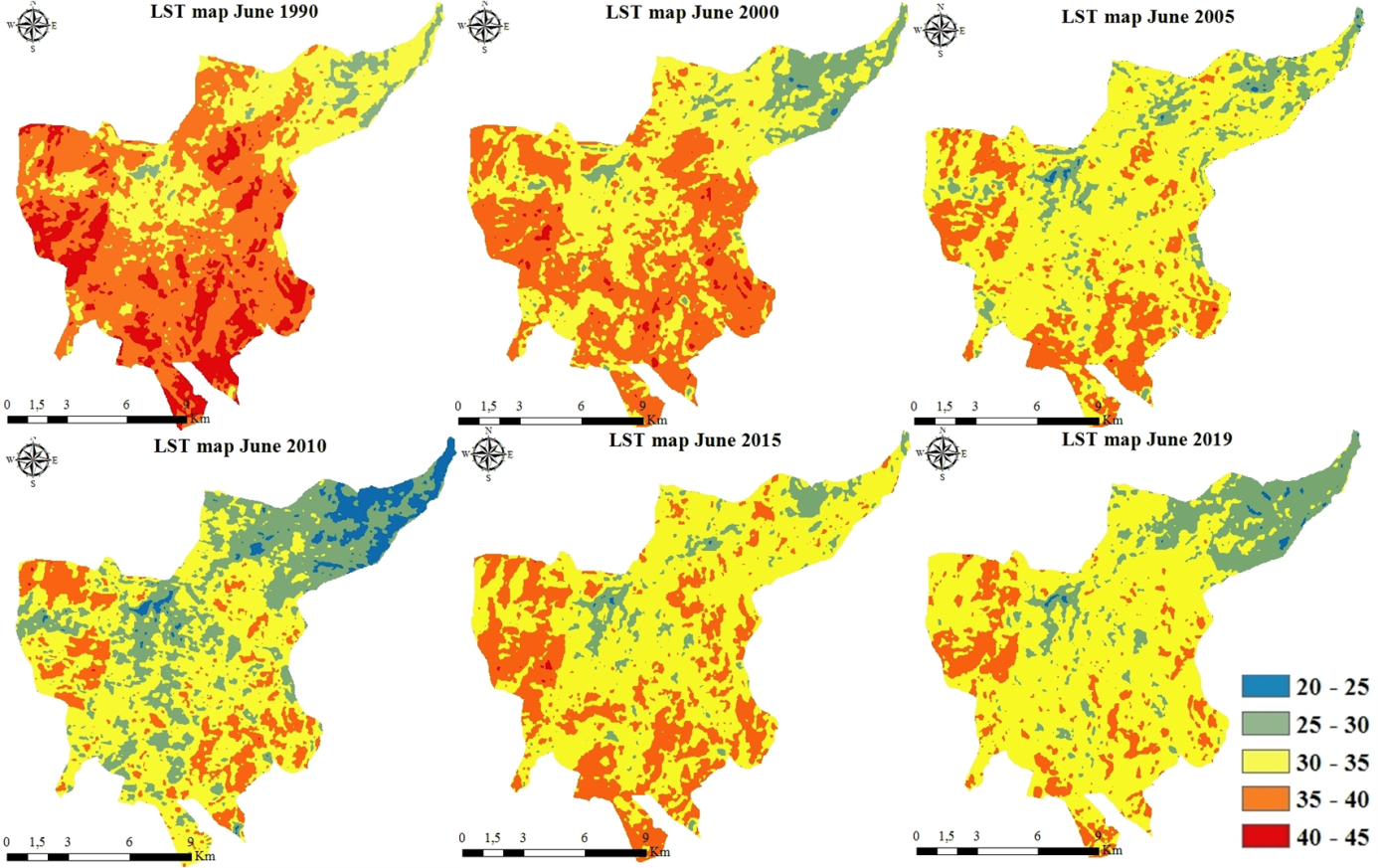
Figure 6: LST maps of June 1990, 2000, 2005, 2010, 2015 and 2019 respectively
3.4 Correlation between NDVI and LST
43According to Mackey (2012), NDVI is a good indicator for calculating the impact of green cover on LST. It revealed that vegetation can significantly reduce the temperature if the NDVI exceeds 0.35 which indicates a negative relationship between the NDVI index and the LST.
44A bivariate correlation analysis and scatter plots were used to determine the relationship between mean LST and NDVI via the software of statistics SAGA 7.4.0 with a number of points N=100000. The recorded results (Table 5) showed that there was a significant and strong negative relationship between NDVI and LST; all the recorded P-values were less than 01%. The coefficient of Person (R) values varied between “0.382 and 0.0709”. Those results confirmed that the increase in NDVI values results in a decrease in LST values (Figure 7).
Table 5: R Values and P-Values of correlation between NDVI/LST in the period 1990-2019
|
N=40680 |
1990 |
2000 |
2005 |
2010 |
2015 |
2019 |
|
Correlation of Pearson R |
0.701 |
0.709 |
0.520 |
0.673 |
0.382 |
0.562 |
|
P-Value |
0.00042 |
0.00084 |
0.00056 |
0.00063 |
0.00022 |
0.00044 |
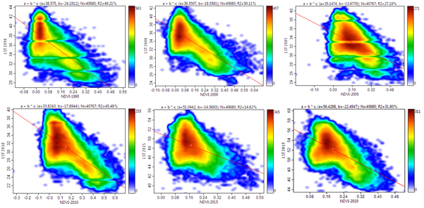
Figure 7: correlation between LST and NDVI of June 1990, 2000, 2005, 2010, 2015 and 2019 respectively.
3.5 Estimation of green cool island effect GCI and urban cool island effect UCI
45The method consists in extracting the mean LST of study area, built-up area, impervious surfaces and each class of vegetation. Using the formulas presented previously, the results obtained were given in Table 6.
Table 6: values of the effect of green cool island GCI and urban cool island UCI
|
June 1990 |
June 2000 |
June 2005 |
June 2010 |
June 2015 |
June 2019 |
|||||||
|
GCI |
UCI |
GCI |
UCI |
GCI |
UCI |
GCI |
UCI |
GCI |
UCI |
GCI |
UCI |
|
|
impervious surfaces |
-5,1 |
3 |
-4,7 |
3,8 |
-3,9 |
3,7 |
-5,3 |
5,8 |
-4,3 |
4,1 |
-5,1 |
4,8 |
|
urban green space |
3,4 |
-5,5 |
4,2 |
-5,1 |
4,4 |
-4,6 |
4,2 |
-3,7 |
4,9 |
-5,1 |
4,6 |
-4,9 |
|
forest D >1000h |
5,6 |
-7,7 |
6,7 |
-7,6 |
7,2 |
-7,4 |
9,3 |
-8,8 |
9,9 |
-10 |
9,6 |
-9,9 |
|
forest D >500h |
2,9 |
-5 |
4 |
-4,9 |
6 |
-6,2 |
4,2 |
-3,7 |
5,8 |
-6 |
4,5 |
-4,9 |
|
forest D >200h |
3,9 |
-6 |
4,8 |
-5,7 |
5,1 |
-5,3 |
5,3 |
-4,8 |
4,9 |
-5,1 |
5,2 |
-5,5 |
|
forest D >100h |
3,7 |
-5,8 |
5 |
-5,9 |
6,4 |
-6,6 |
6,4 |
-5,9 |
6,4 |
-6,3 |
6,3 |
-6,6 |
|
forest D >50h |
6,4 |
-8,5 |
7,3 |
-8,2 |
8,5 |
-8,7 |
8 |
-7,5 |
8,9 |
-9,4 |
8,5 |
-8,8 |
|
forest D ˂50h |
4,4 |
-6,5 |
4,8 |
-5,7 |
6,4 |
-6,6 |
6,7 |
-6,2 |
6,8 |
-7 |
7,4 |
-7,7 |
46The analysis of Table 6 showed that:
47-The forest of Djbel El Ouahch with a density that exceeds 1000h (1050m of altitude) and the forest of Oued Ziad with a density that exceeds 50h had the most important cooling effect. Both Djbel El Ouahch and Oued Ziad forests can generate a cooling effect more than their surroundings with 9.9°C and 8.9°C respectively. They can also affect the urban area with an urban cooling effect of -10°C and -9.4°C respectively.
48-The other forests “Hadji Baba, Meridj, Djebess and Mensourah” had a less important cooling effect than Djbel El Ouahch and Oued Ziad because of their altitude and density.
49-The urban green spaces had a less important cooling effect than forests.
50- Bare soil and impervious surfaces had low values of cooling effect.
3.6 Effects of landscape composition and pattern on land surface temperature
51The land use maps presented the basic data for calculating the landscape metrics using the FRAGSTAT 4.2 software. Several indices used in the analysis of green cover were chosen at the global landscape scale (CA, NP, PD, LPI, LSI, PR and AI) to measure the changes in the green landscape of Constantine city. They were also chosen at the level of each class (CA, PD, PLAND, NP, LPI, LSI, MPS, AI and SHAPE MN) to measure changes in different cover classes. To achieve this, the land use maps were converted to an ASCII file after the extraction of the vegetation class. The study of these metrics has given an idea of the presence and abundance of patches (landscape composition) and the spatial configuration of patches (landscape configuration). The correlation between those metrics and LST was analyzed using SPSS 26 by estimating the Coefficient of Pearson R and P-Values in order to know whether the relationship is significant or not.
3.6.1 Results of landscape metrics at landscape level
The landscape metrics of green cover at landscape level indicated landscape processes from the comparison of the number, richness and diversity of green patches in Constantine city (Table 7).
Table 7: results of landscape metrics at landscape level
|
CA |
NP |
PD |
LPI |
LSI |
PR |
AI |
|
|
1990 |
3995,8200 |
1108,0000 |
27,7290 |
62,1244 |
35,8365 |
1,0000 |
83,3650 |
|
2000 |
3845,6100 |
988,0000 |
25,6916 |
67,9515 |
33,7802 |
1,0000 |
84,0424 |
|
2005 |
4035,0900 |
1211,0000 |
27,5252 |
60,0024 |
36,4435 |
1,0000 |
80,7911 |
|
2010 |
4586,2200 |
1345,0000 |
29,3270 |
61,1386 |
38,2478 |
1,0000 |
83,4069 |
|
2015 |
4376,7900 |
1654,0000 |
37,7903 |
37,4720 |
43,7376 |
1,0000 |
80,4896 |
|
2019 |
5413,8600 |
1859,0000 |
34,3378 |
52,9690 |
43,0367 |
1,0000 |
82,7737 |
52Analysis of the Table 7 showed that Class area (CA), Number of patch (NP), Patch density (PD) and landscape shape index (LSI) increased from 1990 to 2019, despite the constancy of Patch richness (PR) which was always represented by a single class (1).
53The area under vegetation increased gradually from 3995 hectares in 1990 to 5413 hectares in 2019. Both patch density PD and NP generally increased from 1990 to 2019, indicating that patches had become more fragmented in time. Aggregation index (AI) slightly decreased from 1990 to 2019 indicating that the patches had become less aggregated. Largest patch index LPI decreased from 62,12 in 1990 to 52,96 in 2019. This indicates that patches have become smaller and the landscape had become more fragmented. However, the landscape shape index increased from 35, 83 in 1990 to 43,03 in 2019 indicating that landscape had become more complicated. These results have showed that the green landscape of our case study is complicated due to the heterogeneity increase.
3.6.2. Results of landscape metrics at class level
54The recorded results showed that:
55-The values of the surface occupied by a class area (CA) varied between 0.09 hectares and 97.56 hectares with an average of 23.34 hectares. The green patterns were heterogeneous generating a heterogeneous green landscape.
56-The values of percentage of the landscape (PLAND) varied between 0.002 and 0.224.
57-The values of patches number (NP) varied between 1 to 49 patches per class, with an average of 11.54 patches per class. The non-homogeneous distribution of green patches generated a heterogeneous and fragmented landscape.
58-The patches density values per class (PD) varied between 0.0023 and 0.1125, with an average of 0.025.
59-The values of the largest patch index (LPI) varied between 0.0002 and 0.224 with an average of 0.004. So, the green landscape of the city of Constantine was dominated by big green patches (forests with large surface).
60-The values of the Landscape Shape Index (LSI) varied between 1 and 7.34 with an average of 3.46. Whereas, the values of Mean patch shape index (SHAPE_MN) varied between 1 and 2.52 with an average of 1.228. These values expressed the complicated forms of green patterns which composed our landscape.
61-The values of aggregation index (AI) varied between 0 and 100, with an average of 68.83. They had indicated that the green landscape generally consisted of aggregated and adjacent patches which resulted in a fragmented green landscape.
3.6.3. Relationship between green patterns and spatial distribution of LST
62Some studies have confirmed the relationship between spatial characteristics of land use and LST (Zhou et al. 2011, Weng et al. 2007, Liu and Weng 2009). These studies have indicated that landscape metrics retain significant potential in exploring the spatial distribution of the LST. However, most of these studies had examined the effects of spatial characteristics of land use, particularly green cover and built-up areas (Cao et al. 2010, Zhang et al. 2009, Weng et al. 2007), on the LST.
-
Area-related metrics:
63The recorded results indicated that the relationship between the class area CA and LST is a significant negative relationship. The graph showed a linear relationship with R2 = 0.369 and P = 0.000122 (Table 8). The relationship between the class area and the distribution of LST is strong. Similarly for the percentage of landscape PLAND, a significant negative relationship was established with the LST with R2= 0.369 and P =0.000122 (Table 8). This indicates that the increase in the surface and in the percentage of green patches generated the decrease in land surface temperature (LST) (Figure 8).
64-A strong negative relationship was established between Mean patch size MPS and LST with R2= 0.139 and P = 0,000289 (Table 8). The increase in MPS values signified a less fragmented and homogeneous green landscape which helps to lower the land surface temperature LST (Figure 8).
65-We have found that a strong negative relationship was established between the largest patch index LPI and LST with R2= 0.382 and P = 0,000115 (Table 8). The increase in LPI values caused the decrease in LST values, thereby, the dominance of a large green patch helped to reduce LST (Figure 8).
-
Fragmentation and aggregation
66We found that the relationship between the number of patches NP and LST was positive. A significant logarithmic relationship was established with R2= 0.155 and P = 0,000490 (Table 8). Likewise for the density of patches PD with LST, they had a very strong and significant positive relationship with R2= 0.155 and P = 0,000490 (Table 8). These results showed that the fragmentation of green landscape into several green patches caused the increase of LST (Figure 8).
67- For the AI aggregation index, there was a significant negative relationship between AI and LST with R2= 0.225 and P = 0.000202 (Table 8). The high values of AI caused the temperature drop that means adjacent, aggregated and homogeneous green patches were recommended to reduce the LST temperature (Figure 8).
-
Shape complexity
68- A strong positive relationship had been established between LSI and LST, R2= 0.058 and P= 0.000229 (Table 8). The high values of LSI and the complication of green landscape caused the increase in soil surface temperature. So, a well structured and simple landscape was preferable to attenuate the temperature (Figure 8). We found that a significant negative relationship was established between the average index of patches shape (SHAPE_MN) and LST. A weak linear relation with R2= 0.139 and P= 0.000290 (Table 8) as well as the increase in the values of this index caused the reduction of LST (Figure 8).
Table 8: Correlation of Person R and P-Values of different metrics
|
N=228 |
CA |
PLAND |
MPS |
LPI |
PD |
NP |
AI |
SHAPE |
LSI |
|
R |
-0.607 |
-0.607 |
-0.373 |
-0.617 |
0.393 |
0.393 |
-0.474 |
-0.372 |
0.241 |
|
P-Values |
0.000122 |
0.000122 |
0.000289 |
0.000115 |
0.000490 |
0.000490 |
0.000202 |
0.000290 |
0.000229 |
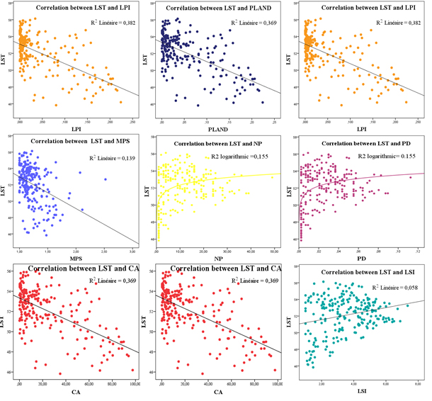
Figure 8: Correlation between LSI and landscape metrics
4. Discussion
69The study confirmed that the impervious surfaces were the warmest areas and they have the highest values of LST during the study period. It also confirmed that the most influential green spaces were the Djbel El Ouahch forest and the Oued Ziad Forest with the most important cooling effect during the study period.
4.1 Relationship between cooling effect / type of vegetation
70Constantine city is a very rich region in green space (the green cover) which varies between deciduous trees, coniferous trees, stem plants, ornamental plants and grass. According to the recorded results of LST and GCI of vegetation; grass, bushes, and trees had very different cooling effects on the urban thermal environment even if they had the same area (LST in high density is lower than LST of grass). So, the vertical distribution of vegetation (the altitude) has to be considered for obtaining a more precise relationship between vegetation characteristics and the urban thermal environment. Even the different types of trees which were located out of the urban area and consume a large amount of water had a good effect because of transpiration compared to the other types of trees (Aleppo pine or Pinus halepensis, Eucalyptus, Cupressus and Quercus suber) that are located in the urban area and Oued Ziad forest.
4.2 Relationship between cooling effect and vegetation density
71The results of this research indicated that the LST and the effect of cooling islands corresponded closely to the distribution of land use characteristics. We confirmed that forest vegetation (at high density) had the most important cooling effect compared to the mean LST of vegetation in the urban area (lowest density). This implied that the cooling effect of the vegetation worked only when the cover reached a certain degree (NDVI> 0.35). They also indicated that a cooling island was the aggregate result of the surrounding colder zones. Also, the cumulative cooling effects of the surrounding green spaces create the zone of maximum temperature reduction in the cooling island.
4.3 Relation spatial patterns and cooling effect
72The metrics for fragmentation and aggregation (PD, NP and AI) showed that the less fragmented (lower PD and NP) and more aggregated (higher AI) green patches, generated lower LST. All landscape metrics were significantly correlated with LST in different degrees. Overall, all Area-related metrics (CA, PLAND, MPS and LPI) were all negatively correlated with LST, suggesting that relatively more green cover with larger patches bring higher cooling effect.
73Shape index complexity metrics LSI was positively correlated with LST and SHAPE_AM was negatively correlated with LST, suggesting that green cover in our study area with simpler shapes and patches were more effective in cooling effect.
74The fragmentation and aggregation metrics (PD, NP and AI) indicated that the less fragmented green landscape (lower PD and NP) and more aggregated green landscape (Higher AI) generate lower LST.
5. Conclusion
75Constantine city contains a variety of green spaces (forests, parks, gardens….) which give it the character of a varied green landscape. In this study, we tried to estimate the impact of spatiotemporal variations of this green cover on the urban climate and the spatial distribution of land surface temperature LST. Remote sensing offered a judicious mean to evaluate this impact through the estimation of NDVI, LST, GCI, UCI indices. A bivariate correlation analysis and scatter plots were used to determine the relationship between the LST and green spaces. The recorded results showed that there is a negative relationship between NDVI and LST, the increase in NDVI values results in a decrease in LST values. In addition, the obtained results indicated that the LST and the cooling effect of green spaces corresponded closely to the distribution of land use characteristics. Dense green spaces with the highest values of NDVI have the highest cooling effect. Thus, our study confirmed that the type and density of vegetation as well as the size and shape of green spaces were all important factors in determining the cooling effect. It was an effective means to mitigate the urban heat island effect UHI, reduce the effects of heat stress and provide a comfortable outdoor environment for users.
76Linking the remote sensing and the theory of landscape metrics, the correlation between landscape metrics and LST was studied by using SPSS 26. Our results confirmed that both the composition and the configuration of green spaces have a significant and strong relationship with the spatial distribution of LST where R2 varied between (0.052 and 0.382) and P-values varied between (0.000115 and 0.000490). The results revealed that a simple, homogeneous and aggregated green landscape was more efficient. The large dominant green patch had the highest impact on LST and the most fragmented green patch with complicated shapes led to an increase in LST.
77At the end of this study, it should be noted that the vegetation cover in the city of Constantine is a cover to be restructured especially within an urban area, particularly the choice of the type and the size of this cover. Giving an importance to the surrounding forests makes them more effective to mitigate urban heat island (UHI).
6. References
78Ali-Khodja A. (2011), Espace vert public urbain: de l'historicisme à la normativité, Thèse de Doctorat, Département d’Architecture et d’Urbanisme, Faculté des Sciences de la Terre et de l’Aménagement du Territoire, Université Mentouri Constantine.
79Boudjellal, L., & Bourbia, F. (2018). An evaluation of the cooling effect efficiency of the oasis structure in a Saharan town through remotely sensed data. International Journal of Environmental Studies, 75(2), 309-320.
80Bounoua, L., Hall, F. G., Sellers, P. J., Kumar, A., Collatz, G. J., Tucker, C. J., & Imhoff, M. L. (2010). Quantifying the negative feedback of vegetation to greenhouse warming: A modeling approach. Geophysical Research Letters, 37(23).
81Cao, X., Onishi, A., Chen, J., & Imura, H. (2010). Quantifying the cool island intensity of urban parks using ASTER and IKONOS data. Landscape and urban planning, 96(4), 224-231.
82Chatzidimitriou, A., Chrissomallidou, N., & Yannas, S. (2006, September). Ground surface materials and microclimates in urban open spaces. In PLEA2006–The 23rd Conference on Passive and Low Energy Architecture, Geneva (p. 6).
83Chun, B., & Guldmann, J. M. (2018). Impact of greening on the urban heat island: Seasonal variations and mitigation strategies. Computers, Environment and Urban Systems, 71, 165-176. Yu, C., & Hien, W. N. (2006). Thermal benefits of city parks. Energy and buildings, 38(2), 105-120.
84Cohen, P., Potchter, O., & Matzarakis, A. (2012). Daily and seasonal climatic conditions of green urban open spaces in the Mediterranean climate and their impact on human comfort. Building and Environment, 51, 285-295.
85Fintikakis, N., Gaitani, N., Santamouris, M., Assimakopoulos, M., Assimakopoulos, D. N., Fintikaki, M., & Doumas, P. (2011). Bioclimatic design of open public spaces in the historic centre of Tirana, Albania. Sustainable Cities and Society, 1(1), 54-62.
86Gherraz, H., Guechi, I., & Benzaoui, A. (2018). Strategy to improve outdoor thermal comfort in open public space of a Desert City, Ouargla, Algeria. In IOP Conference Series: Earth and Environmental Science (Vol. 151).
87Giridharan, R., Lau, S. S. Y., Ganesan, S., & Givoni, B. (2008). Lowering the outdoor temperature in high-rise high-density residential developments of coastal Hong Kong: The vegetation influence. Building and Environment, 43(10), 1583-1595.
88Guo, Z., Wang, S. D., Cheng, M. M., & Shu, Y. (2012). Assess the effect of different degrees of urbanization on land surface temperature using remote sensing images. Procedia Environmental Sciences, 13, 935-942.
89Hamada, S., & Ohta, T. (2010). Seasonal variations in the cooling effect of urban green areas on surrounding urban areas. Urban forestry & urban greening, 9(1), 15-24.
90Hanafi, A., & Alkama, D. (2017). Role of the urban vegetal in improving the thermal comfort of a public place of a contemporary Saharan city. Energy Procedia, 119, 139-152.
91Du, H., Cai, W., Xu, Y., Wang, Z., Wang, Y., & Cai, Y. (2017). Quantifying the cool island effects of urban green spaces using remote sensing Data. Urban Forestry & Urban Greening, 27, 24-31.
92Jusuf, S. K., Wong, N. H., Hagen, E., Anggoro, R., & Hong, Y. (2007). The influence of land use on the urban heat island in Singapore. Habitat international, 31(2), 232-242.
93Kong, F., Yin, H., James, P., Hutyra, L. R., & He, H. S. (2014). Effects of spatial pattern of greenspace on urban cooling in a large metropolitan area of eastern China. Landscape and Urban Planning, 128, 35-47.
94Landsberg, H. E. (1981). The urban climate. Academic press.
95Liu, H., & Weng, Q. (2009). Scaling effect on the relationship between landscape pattern and land surface temperature. Photogrammetric Engineering & Remote Sensing, 75(3).
96Mackey, C. W., Lee, X., & Smith, R. B. (2012). Remotely sensing the cooling effects of city scale efforts to reduce urban heat island. Building and Environment, 49, 348-358.
97Maheng, D., Ducton, I., Lauwaet, D., Zevenbergen, C., & Pathirana, A. (2019). The Sensitivity of Urban Heat Island to Urban Green Space—A Model-Based Study of City of Colombo, Sri Lanka. Atmosphere, 10(3), 151.
98McGarigal, K., Compton, B., Jackson, S. D., Rolih, K., & Ene, E. (2005). Conservation assessment a prioritization system (CAPS). Final report. Landscape ecology program. Department of Natural Resources Conservation, University of Massachusetts, USA.
99Miller, R. W., Hauer, R. J., & Werner, L. P. (2015). Urban forestry: planning and managing urban greenspaces. Waveland press.
100Oliveira, S., Andrade, H., & Vaz, T. (2011). The cooling effect of green spaces as a contribution to the mitigation of urban heat: A case study in Lisbon. Building and environment, 46(11), 2186-2194.
101Parker, D. E. (2010). Urban heat island effects on estimates of observed climate change. Wiley Interdisciplinary Reviews: Climate Change, 1(1), 123-133.
102Qiu, G. Y., Zou, Z., Li, X., Li, H., Guo, Q., Yan, C., & Tan, S. (2017). Experimental studies on the effects of green space and evapotranspiration on urban heat island in a subtropical megacity in China. Habitat international, 68, 30-42.
103Shahidan, M. F., Salleh, E., & Shariff, K. M. (2007). Effects of tree canopies on solar radiation filtration in a tropical microclimatic environment. In PLEA 2007 conference. Singapore (Vol. 18).
104Sorensen, M., Smit, J., Barzetti, V., & Williams, J. (1997). Good practices for urban greening. Inter-American Development Bank.
105Taha, H., Akbari, H., Rosenfeld, A., & Huang, J. (1988). Residential cooling loads and the urban heat island—the effects of albedo. Building and environment, 23(4), 271-283.
106Tan, M., & Li, X. (2013). Integrated assessment of the cool island intensity of green spaces in the mega city of Beijing. International journal of remote sensing, 34(8), 3028-3043.
107United Nations. (2011). World Urbanization Prospects the Revision. Department of Economic and Social Afairs, Population Division.NewYork, 2011.
108Weier J., Herring D. (2000). Measuring vegetation (NDVI & EVI), https://earthobservatory.nasa.gov/Features/MeasuringVegetation
109Weng, Q., Liu, H., & Lu, D. (2007). Assessing the effects of land use and land cover patterns on thermal conditions using landscape metrics in city of Indianapolis, United States. Urban ecosystems, 10(2), 203-219.
110Wu, W. (2014). The generalized difference vegetation index (GDVI) for dryland characterization. Remote Sensing, 6(2), 1211-1233.
111Zhang, X., Zhong, T., Feng, X., & Wang, K. (2009). Estimation of the relationship between vegetation patches and urban land surface temperature with remote sensing. International Journal of Remote Sensing, 30(8), 2105-2118.
112Zhang, Y., Zhan, Y., Yu, T., & Ren, X. (2017). Urban green effects on land surface temperature caused by surface characteristics: A case study of summer Beijing metropolitan region. Infrared Physics & Technology, 86, 35-43.
113Zhou, W., Huang, G., & Cadenasso, M. L. (2011). Does spatial configuration matter? Understanding the effects of land cover pattern on land surface temperature in urban landscapes. Landscape and urban planning, 102(1), 54-63.